Example problem setting

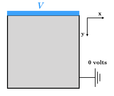
Example (1) Solve Laplace's equation. As shown in the figure, the boundary condition is \ phi = V volt at y = 0. It is grounded at the other boundary and is 0 volt. The electrostatic position at this time is determined and visualized.

Example (2) Solve Poisson's equation. Put the external charge Q in the area considered in Example (1). At this time, the electrostatic potential $ \ phi $ and the electric field $ E =-\ nabla \ phi $ are obtained and visualized.

Example (1) Poisson's equation

Animation is also generated in the code. This is to investigate how the solution \ phi (x, y) converges.

Postscript December 17, 2017: It is supposed to work on jupyter. If you don't use jupyter, comment out "% matplotlib nbagg" in your code. From masa_stone22's point.

laplace.py3

"""
Laplace equation:Numerical solution,Jacobi(Jacobi)Law: 
12 Aug. 2017
"""
%matplotlib nbagg 
import numpy as np
import matplotlib.pyplot as plt
from matplotlib.animation import ArtistAnimation #Import methods for creating animations

fig = plt.figure()
anim = [] 

# 
delta_L=0.1  #Grid width
LL = 10 #Square width
L = int(LL/delta_L)

V = 5.0 #Boundary potential on one side
convegence_criterion = 10**-3  #Convergence condition. Decrease this value to improve accuracy.

phi = np.zeros([L+1,L+1])
phi[0,:] = V #boundary condition
phi2 = np.empty ([L+1,L+1])

#for plot
im=plt.imshow(phi,cmap='hsv')
anim.append([im])

    
#Main
delta = 1.0
n_iter=0
conv_check=[]
while delta > convegence_criterion:
    if n_iter % 100 ==0:  #Monitoring of convergence status
        print("iteration No =", n_iter, "delta=",delta)
    conv_check.append([n_iter, delta])
    for i in range(L+1):
        for j in range(L+1):
            if i ==0 or i ==L or j==0 or j==L:
                phi2[i,j] = phi[i,j]
            else: 
                phi2[i,j] = (phi[i+1,j] + phi[i-1,j] + phi[i,j+1] + phi[i,j-1])/4 #Addendum:formula(11)See
    delta = np.max(abs(phi-phi2))

    phi, phi2 = phi2, phi
    n_iter+=1
    
    im=plt.imshow(phi,cmap='hsv')
    anim.append([im])

#for plot        
plt.colorbar () #Color bar display
plt.xlabel('X')
plt.ylabel('Y')
ani = ArtistAnimation(fig, anim, interval=100, blit=True,repeat_delay=1000)
ani.save("t.gif", writer='imagemagick')  
plt.show()

Result (1) Solution of Laplace's equation

The boundary condition $ \ phi = 5 $ for y = 0 is satisfied. The change in potential is large near the boundary.

Example (2) Solution of Poisson's equation when an external charge is embedded

The external charge density is $ c = 1000 $, and the boundary potential is $ V = 5 $.

Poisson.py3

"""
Poisson equation:Jacobi(Jacobi)Law
Also displays the electric field: 
12 Aug. 2017
"""
%matplotlib nbagg 
import numpy as np
import matplotlib.pyplot as plt
from matplotlib.animation import ArtistAnimation #Import methods for creating animations

anim = [] 

# 
delta_L=0.01 #Grid width
LL = 1 #Square width
L = int(LL/delta_L)

V = 5.0 #Boundary y=0 potential(boundary condition)
convegence_criterion = 10**-5

phi = np.zeros([L+1,L+1])
phi[0,:] = V #boundary condition
phi2 = np.empty ([L+1,L+1])

#Charge density setting
eps0=1
charge= np.zeros([L+1,L+1])
c=1000 #Charge density

CC=int(L/4)
CC2=int(L/2)

#Charge density x=[L/4, L/2], y=[L/4,L/2]Embed in the area of
for i in range(CC, CC2+1):
    for j in range(CC,CC2+1):
        charge[i,j] = c
#

#for plot
im=plt.imshow(phi,cmap='hsv')
anim.append([im])

    
#Main
delta = 1.0
n_iter=0
conv_check=[]
while delta > convegence_criterion:
    if n_iter % 100 ==0:  #Monitoring of convergence status
        print("iteration No =", n_iter, "delta=",delta)
    conv_check.append([n_iter, delta])
    for i in range(L+1):
        for j in range(L+1):
            if i ==0 or i ==L or j==0 or j==L:
                phi2[i,j] = phi[i,j]
            else: 
                phi2[i,j] = (phi[i+1,j] + phi[i-1,j] + phi[i,j+1] + phi[i,j-1])/4 + (delta_L**2/(4*eps0))*charge[i,j]
    delta = np.max(abs(phi-phi2))

    phi, phi2 = phi2, phi
    n_iter+=1
    
    im=plt.imshow(phi,cmap='hsv')
    anim.append([im])

    
#for plot    

pp=plt.colorbar (orientation="vertical") #Color bar display
pp.set_label("phi", fontname="Ariel", fontsize=24)
plt.xlabel('X',fontname="Ariel", fontsize=24)
plt.ylabel('Y',fontname="Ariel", fontsize=24)
plt.title('Solution of the Poisson equation for electrostatic potential ')
#ani = ArtistAnimation(fig, anim, interval=10, blit=True,repeat_delay=1000)
#ani.save("t.gif", writer='imagemagick')  

plt.show()



#Electric field calculation
Ex = np.zeros([L,L])
Ey = np.zeros([L,L])

for i in range(L):
    for j in range(L):
        Ex[i,j] = -(phi[i+1,j]-phi[i,j])/delta_L
        Ey[i,j] = -(phi[i,j+1]-phi[i,j])/delta_L

plt.figure()
        
X, Y= np.meshgrid(np.arange(0, L,1), np.arange(0, L,1))  #Mesh generation
plt.quiver(X,Y,Ex,Ey,color='red',angles='xy',scale_units='xy', scale=40) #Plot vector field

plt.xlim([0,L]) #Range of X to draw
plt.ylim([0,L]) #Range of y to draw

#Graph drawing
plt.grid()
plt.draw()
plt.show()

Result (2): Solution of Poisson's equation of the system with embedded external charge

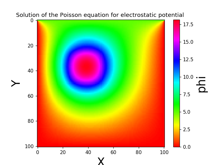
The boundary condition at y = 0 is $ \ phi = 5 $. Due to the embedded external charge, the potential differs greatly compared to Example (1).

The state of the electric field. (The #y axis has been reversed). This figure was drawn as delta_L = 0.1. As expected from the fluctuation of the potential, the electric field fluctuates greatly near the external charge.

Addendum

Addendum (1): Theory

The relational expression between the electrostatic field $ E $ and the potential $ \ phi $ E = - \nabla \phi \tag{1} And Gauss's law between the charge densities $ \ rho $ and $ E $

\nabla \cdot E =\frac{\rho} {\epsilon_0} \tag{2}

Is the starting point.

Substituting (1) into (2)

\Delta \phi (x,y,z) =-\frac{\rho (x,y,z)} {\epsilon_0} \tag{3}

To get. This is the Poisson equation. Where $ \ epsilon_0 $ is the permittivity in vacuum.

If there is no true electric charge everywhere in space ($ \ rho (x, y, z) = 0 $), the Poisson equation is

\Delta \phi (x,y,z) =0 \tag{4} Will be. This is the Laplace equation.

Addendum (2): Numerical solution: Jacobi method

Think two-dimensional. Poisson's equation

$ \frac{\partial^2 \phi(x,y)}{\partial x^2} + \frac{\partial^2 \phi(x,y)}{\partial y^2} =-\frac{\rho (x,y,z)} {\epsilon_0} \tag{5}$

Will be. Consider a two-dimensional grid (see figure below) separated by a width of $ \ Delta $ in the $ x $ and $ y $ directions. Taylor expansion of the potential $ \ phi (x, y) $ at the point ($ x + \ Delta, y $)

\phi(x+\Delta,y)=\phi(x,y)+\frac{\partial \phi}{\partial x}\Delta +\frac{1}{2}\frac{\partial^2 \phi}{\partial x^2}\Delta^2 + \frac{1}{6}\frac{\partial^3 \phi}{\partial x^3}\Delta^3+\frac{1}{24}\frac{\partial^4 \phi}{\partial x^4}\Delta^4 + \mathcal{O}(\Delta^5) \tag{6}

\phi(x-\Delta,y)=\phi(x,y)-\frac{\partial \phi}{\partial x}\Delta +\frac{1}{2}\frac{\partial^2 \phi}{\partial x^2}\Delta^2 - \frac{1}{6}\frac{\partial^3 \phi}{\partial x^3}\Delta^3+\frac{1}{24}\frac{\partial^4 \phi}{\partial x^4}\Delta^4 + \mathcal{O}(\Delta^5) \tag{7}

When Eqs. (6) and Eq. (7) are added together,

$\frac{\partial^2 \phi(x,y)}{\partial x^2} = \frac{\phi(x+\Delta,y)+ \phi(x-\Delta,y)-2\phi(x,y)}{\Delta^2} +\mathcal{O}(\Delta^2) \tag{8} $

Taylor expansion is done for y in the same way, $\frac{\partial^2 \phi(x,y)}{\partial y^2} = \frac{\phi(x,y+\Delta)+ \phi(x,y-\Delta)-2\phi(x,y)}{\Delta^2} +\mathcal{O}(\Delta^2) \tag{9} $

To get. Substitute equations (8) and (9) into (5) and sort them out a little.

$ \phi(x,y) = \frac{1}{4} [\phi(x+\Delta,y)+\phi(x-\Delta,y)+\phi(x,y+\Delta)+\phi(x,y-\Delta)]+\frac{\rho(x,y)}{4 \epsilon_0}\Delta^2+\mathcal{O}(\Delta^4) \tag{10} $

To get. This is a ** differential representation of Poisson's equation **. The error is $ \ mathcal {O} (\ Delta ^ 4) $.

When $ \ rho (x, y) = 0 $

$\phi(x,y) = \frac{1}{4} [\phi(x+\Delta,y)+\phi(x-\Delta,y)+\phi(x,y+\Delta)+\phi(x,y-\Delta)]+\mathcal{O}(\Delta^4) \tag{11} $

Will be. This is a ** differential representation of Laplace's equation **.

In numerical calculation, if the subscript of the array is $ (x_i, y_j) $, equation (10) is

$ \phi(x_i,y_j) = \frac{1}{4} [\phi(x_{i+1},y_{j})+\phi(x_{i-1},y_{j})+\phi(x_{i},y_{j+1})+\phi(x_{i},y_{j-1})]+\frac{\rho(x_{i},y_{j})}{4\epsilon_0}\Delta^2　\tag{12} $ Will be.

The potential $ \ phi (i, j) $ at the point $ (x_i, y_j) $ is approximated by adding the amount proportional to the charge density $ \ rho (x, y) $ to the average value of the values of the surrounding four points. Is done (see the figure below).

** First, give the boundary conditions and the estimated value of the potential in the region, solve Eq. (12) in all regions, and repeat until the solutions in the region converge. This is the Jacobi method. ** The number of repeating steps for convergence is approximately proportional to the square of the number of data points [1].

This method is very slow to converge and impractical, but it provides a basis for understanding modern methods.

References

The Jacobi method and a slightly modified good calculation method [Gauss-Seidel method](https://ja.wikipedia.org/wiki/%E3%82%AC%E3%82%A6%E3%82% B9% EF% BC% 9D% E3% 82% B6% E3% 82% A4% E3% 83% 87% E3% 83% AB% E6% B3% 95) is slow to converge and impractical. Faster schemes include Sequential Over-relaxation (SOR) [1,2].

[1] ["Numerical Recipe in Sea Japanese Version-Recipe for Numerical Calculation in C Language"](https://www.amazon.co.jp/%E3%83%8B%E3%83%A5 % E3% 83% BC% E3% 83% A1% E3% 83% AA% E3% 82% AB% E3% 83% AB% E3% 83% AC% E3% 82% B7% E3% 83% 94-% E3% 82% A4% E3% 83% B3-% E3% 82% B7% E3% 83% BC-% E6% 97% A5% E6% 9C% AC% E8% AA% 9E% E7% 89% 88- C% E8% A8% 80% E8% AA% 9E% E3% 81% AB% E3% 82% 88% E3% 82% 8B% E6% 95% B0% E5% 80% A4% E8% A8% 88% E7% AE% 97% E3% 81% AE% E3% 83% AC% E3% 82% B7% E3% 83% 94-Press-William-H / dp / 4874085601 / ref = dp_return_1? _ Encoding = UTF8 & n = 465392 & s = books) Technical Review, 1993.

As something that can be viewed on the net

http://www.na.scitec.kobe-u.ac.jp/~yamamoto/lectures/appliedmathematics2006/chapter8.PDF

When

http://web.econ.keio.ac.jp/staff/ito/pdf02/pde2.pdf

I will list.

Postscript: August 14, 2017

I posted an article about SOR method and Gauss-Seidel method.

[2] Qiita article, [[Science and technology calculation by Python] Comparison of convergence speeds of Jacobi method, Gauss-Seidel method, and SOR method for Laplace equation, partial differential equation, boundary value problem, numerical calculation](http: // qiita.com/sci_Haru/items/b98791f232b93690a6c3)

Addendum: ** Code for solving Poisson's equation by SOR method **

The code to solve the Poisson's equation in Example (2) by the SOR method explained in the article [2] is posted. Converges more than 10 times faster than the Jacobi method </ font>, so use this.

"""
Poisson equation:Numerical solution,SOR method
Also displays the electric field:
14 Aug. 2017
"""
%matplotlib nbagg 
import numpy as np
import matplotlib.pyplot as plt
from matplotlib.animation import ArtistAnimation #Import methods for creating animations
import matplotlib.animation as animation


anim = [] 

# 
delta_Lx=0.01
delta_Ly=0.01
LLx = 1 #Square width
LLy= 1

Lx = int(LLx/delta_Lx)
Ly = int(LLy/delta_Ly)



V = 5.0 #Voltage
convegence_criterion = 10**-5

phi = np.zeros([Lx+1,Ly+1])
phi_Bound= np.zeros([Lx+1,Ly+1])
phi_Bound[0,:] = V #boundary condition

#Charge density setting
eps0=1
charge= np.zeros([Lx+1,Ly+1])
c=1000

CC=int(Lx/4)
CC2=int(Ly/2)

for i in range(CC, CC2+1):
    for j in range(CC,CC2+1):
        charge[i,j] = c
#


# for SOR method
aa_recta=0.5*(np.cos(np.pi/Lx)+np.cos(np.pi/Ly))
omega_SOR_recta = 2/(1+np.sqrt(1-aa_recta**2)) #Acceleration parameters in SOR method
print("omega_SOR_rect=",omega_SOR_recta)



#for plot
im=plt.imshow(phi,cmap='hsv')
anim.append([im])

    
#Main
delta = 1.0
n_iter=0
conv_check=[]
while delta > convegence_criterion:
    phi_in=phi.copy()
    if n_iter % 100 ==0:  #Monitoring of convergence status
        print("iteration No =", n_iter, "delta=",delta)
    conv_check.append([n_iter, delta])
    for i in range(Lx+1):
        for j in range(Ly+1):
            if i ==0 or i ==Lx or j==0 or j==Ly:
                phi[i,j] = phi_Bound[i,j]
            else: 
                phi[i,j] = phi[i,j]+omega_SOR_recta *((phi[i+1,j] + phi[i-1,j] + phi[i,j+1] + phi[i,j-1])/4-phi[i,j]+ (delta_Lx*delta_Ly/(4*eps0))*charge[i,j]) # SOR =Gauss-Seidel+ OR
    delta = np.max(abs(phi-phi_in))


    n_iter+=1
    
    im=plt.imshow(phi,cmap='hsv')
    anim.append([im])

    
#for plot    

pp=plt.colorbar (orientation="vertical") #Color bar display
pp.set_label("phi", fontname="Ariel", fontsize=24)
plt.xlabel('X',fontname="Ariel", fontsize=24)
plt.ylabel('Y',fontname="Ariel",  fontsize=24)
plt.title('Solution of the Poisson equation for electrostatic potential ')
#ani = ArtistAnimation(fig, anim, interval=10, blit=True,repeat_delay=1000)
#ani.save("t.gif", writer='imagemagick')  

plt.show()



#Electric field calculation
Ex = np.zeros([Lx,Ly])
Ey = np.zeros([Lx,Ly])

for i in range(Lx):
    for j in range(Ly):
        Ex[i,j] = -(phi[i+1,j]-phi[i,j])/delta_Lx
        Ey[i,j] = -(phi[i,j+1]-phi[i,j])/delta_Ly

plt.figure()

X, Y= np.meshgrid(np.arange(0, Lx,1), np.arange(0, Ly,1))  #Mesh generation
plt.quiver(X,Y,Ex,Ey,color='red',angles='xy',scale_units='xy', scale=40) #Plot vector field

plt.xlim([0,Lx]) #Range of X to draw
plt.ylim([0,Ly]) #Range of y to draw

#Graph drawing
plt.grid()
plt.draw()
plt.show()