2. Multivariate analysis spelled out in Python 7-3. Decision tree [regression tree]

• Another aspect of the decision tree, ** regression tree ** with the objective variable as numerical data.
• For the ** classification tree ** whose objective variable is categorical data, use the ** DecisionTreeClassifier ** of the scikit-learn.tree module, but for the ** regression tree ** model, use ** DecisionTreeRegressor **.

⑴ Import library

import numpy as np
import pandas as pd
import matplotlib.pyplot as plt

from sklearn.tree import DecisionTreeRegressor #A class that creates a regression tree model

⑵ Data acquisition and reading

from sklearn.datasets import load_boston
boston_dataset = load_boston()

• For data, use the "Boston house prices dataset" that comes with scikit-learn.
• There are 13 features and 506 samples related to the housing situation in Boston, a large city in the northeastern United States.
• The aim of this dataset is to predict home prices using given features.
• The target is the price of the house with the variable name MEDV (abbreviation of Median value), and the 13 features are explanatory variables for predicting the price of the house.
• Click here for details such as the contents of explanatory variables https://qiita.com/y_itoh/items/aaa2056aac0c270ba7d2

** Build a regression tree model that predicts the price of a house using the 13 explanatory variables that characterize the house. ** **

• First, convert 13 explanatory variables to a data frame.

#Store explanatory variables in DataFrame
boston = pd.DataFrame(boston_dataset.data, columns=boston_dataset.feature_names)

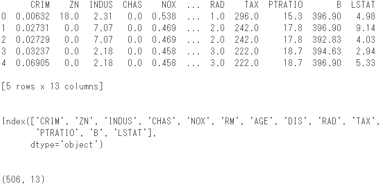
print(boston.head()) #Display the first 5 lines
print(boston.columns) #Show column name
print(boston.shape) #Check the shape

• Add the objective variable there as column name MEDV.

#Add objective variable
boston['MEDV'] = boston_dataset.target

print(boston.head()) #Display the first 5 lines
print(boston.shape) #Reconfirm the shape

• The number of samples is 14 columns by adding the objective variable to the explanatory variables of 506 and 13.
• Randomly divide this dataset into two groups, a training dataset and a test dataset.

⑶ Data division

#Convert dataset to Numpy array
array = boston.values

#Divide into explanatory variables and objective variables
X = array[:,0:13]
Y = array[:,13]

• 70% of the data is used as training data, and the remaining 30% is used as test data.

#Import module to split data
from sklearn.model_selection import train_test_split

#Split data
X_train, X_test, Y_train, Y_test = train_test_split(X, Y, test_size=0.3, random_state=1234)

⑷ Construction of regression tree model

• As with the classification tree, we pass the arrays X and Y to the fit method for training, but in this case Y is a numeric type.
• The optional max_leaf_nodes specifies how much the tree will grow. Here, the maximum number of leaf nodes is 20.

#Model instantiation
reg = DecisionTreeRegressor(max_leaf_nodes = 20)

#Model generation by learning
model = reg.fit(X_train, Y_train)
print(model)

⑸ Evaluation of regression tree model

• The resulting regression tree model is tested from two directions: the validity of the prediction (➀) and the versatility of the model itself (➁).
• First, in order to confirm the validity of the prediction, one is randomly selected from 506 samples, and the price predicted from the feature quantity is compared with the actually observed price.

➀ Confirm the validity of the forecast

• Randomly retrieve only one id from the original dataset X.

#Import Python standard pseudo-random number module
import random
random.seed(1)

#Randomly select id
id = random.randrange(0, X.shape[0], 1)
print(id)

#Extract the relevant sample from the original dataset
x = X[id]
x = x.reshape(1,13)

#Predict house prices from explanatory variables
YHat = model.predict(x)

#Convert the explanatory variable of the id to DataFrame
df = pd.DataFrame(x, columns = boston_dataset.feature_names)
#Added predicted value y
df["Predicted Price"] = YHat

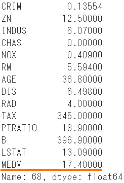
• Get the actually observed home prices and compare them.

boston.iloc[id]

• The expected price is 20.45, compared to the actual price of 17.40.
• The next verification is how much the predicted value of the model can explain the amount of information of the observed value.

➁ Check the coefficient of determination as an indicator of versatility

• The coefficient of determination $ R ^ 2 $ is an index that expresses the explanatory power of the predicted value $ \ hat {y} $ for the observed value $ y $ in regression analysis, and is also called the contribution rate.
• Takes a value from 0 to 1, and the closer $ R ^ 2 $ is to 1, the more valid the model.

#Import the function to calculate the coefficient of determination
from sklearn.metrics import r2_score

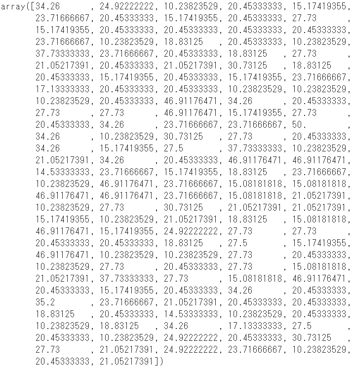
• Pass the explanatory variable for testing (X_test) to the model to calculate the predicted value.

YHat = model.predict(X_test)

• Pass these predictions and the test objective variable (Y_test) to calculate the coefficient of determination.

r2 = r2_score(Y_test, YHat)
print("R^2 = ", r2)

• The goodness of fit of the model in the test data is 0.86, which is a good result.

⑹ Visualization of regression tree model

#Import sklearn tree module
from sklearn import tree

#Module to display images in Notebook
from IPython.display import Image

#Module for visualizing decision tree model
import pydotplus

#Convert decision tree model to DOT data
dot_data = tree.export_graphviz(model,
                                out_file = None,
                                feature_names = boston_dataset.feature_names,
                                class_names = 'MEDV',
                                filled = True)

#Draw a diagram
graph = pydotplus.graph_from_dot_data(dot_data)  

#View diagram
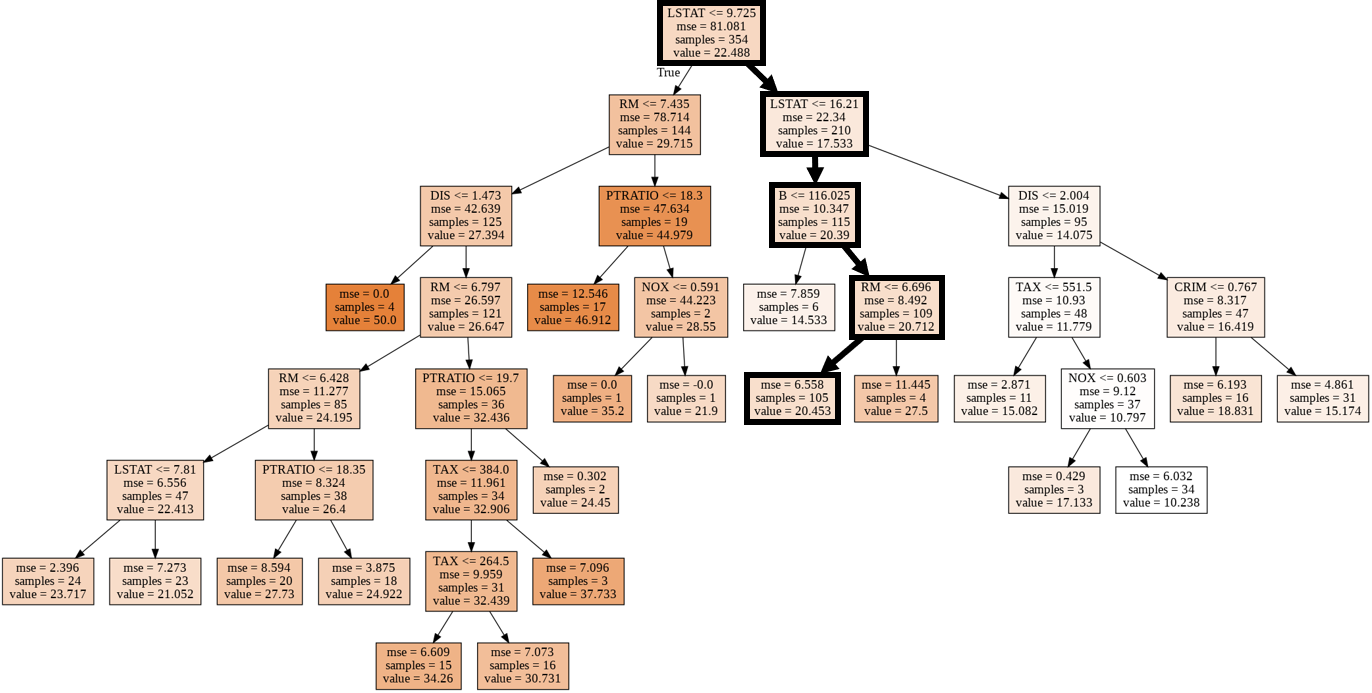
Image(graph.create_png())

• The route of the randomly extracted sample (ID: 68) is shown by a thick line.
• By the way, the feature quantity "LSTAT" of the parent node and the child node of the first layer is an abbreviation of "lower status" and means the ratio of the lower class to the population.