[PYTHON] Investigate the effect of outliers on correlation

Today, I used pandas to refer to the contents of Chapter 10 "Effects of Outliers on Correlation Coefficients" in Easy Statistics by R. I will explain how to remove outliers while examining the correlation. The original book used R, but pandas can be an alternative to easily perform dataframe-based analysis in Python.

Examine animal weight and brain weight

As in the original book [Data on animal weight and weight](http://www.open.edu/openlearn/science-maths-technology/mathematics-and-statistics/mathematics/exploring-data-graphs-and- Use numerical-summaries / content-section-2.7).

First of all, I prepared this as CSV data so that it can be handled by a computer like the other day (https://github.com/ynakayama/sandbox/blob) /c4720fb8ff2973314e06e8cd2342b0e8e849889f/python/pandas/animal.csv).

Bring CSV data into a data frame.

animal = pd.read_csv('animal.csv')

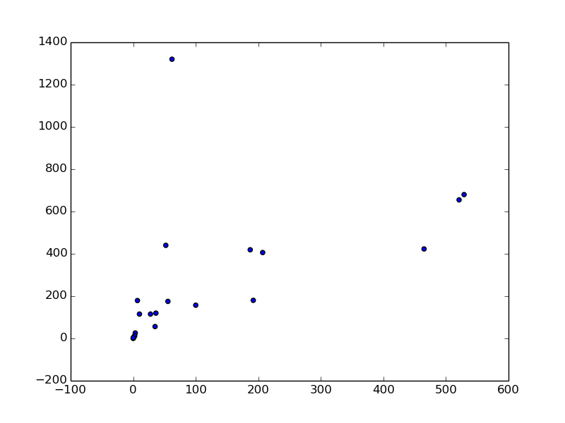
Draw a scatter plot to find the correlation coefficient

If you have two variables and want to examine their correlation, the first step is to look at a scatter plot. How to draw a scatter plot is as explained before. I'll try it right away.

plt.figure()
plt.scatter(animal.ix[:,1], animal.ix[:,2])
plt.savefig('animal.png')

Then find the correlation coefficient as usual.

animal.corr()
#=>
#                   Body weight (kg)  Brain weight (g)
# Body weight (kg)          1.000000         -0.005341
# Brain weight (g)         -0.005341          1.000000

The value of the correlation coefficient -0.005 was obtained as shown on page 250 of the original book. At this rate, there is almost no correlation.

Remove outliers

The method of checking outliers is as described in I explained before, but the outliers are identified and removed according to the R code of the original book. To go. First, there is only one dot on the right side of the scatter plot above. This is a Brachiosaurus dinosaur called Brachiosaurus at number 24 in Data and weighs 80,000 kg. The data shows that the brain weighs less than 1,000 g. Let's get rid of this.

#Select only data that weigh less than 80,000
animal2 = animal[animal.ix[:,1] < 80000]

This means selecting data that weighs less than 80,000. If you do not add an index reference, only less than 80000 of the data will remain, and the data that does not correspond will be NaN. Therefore, even if you write this, the result is the same.

animal2 = animal[animal < 80000].dropna()

In this state, draw a scatter plot and find the correlation coefficient.

animal2.corr()
#=>
#                   Body weight (kg)  Brain weight (g)
# Body weight (kg)          1.000000          0.308243
# Brain weight (g)          0.308243          1.000000

The correlation coefficient is now 0.30. There will be a slightly weaker positive correlation. In addition, as in the original book, let's remove four animals that weigh more than 2,000 kg.

animal2 = animal[animal.ix[:,1] < 2000]
animal2.corr()
#=>
#                   Body weight (kg)  Brain weight (g)
# Body weight (kg)          1.000000          0.542351
#Brain weight (g)          0.542351          1.000000

plt.scatter(animal2.ix[:,1], animal2.ix[:,2])

This time the correlation coefficient has risen to 0.54. You can see that there is only one outlier in the upper left of the scatter plot. It is a human, weighing less than 100 kg and weighing more than 1,200 g in the brain. It can be seen that the ratio of the weight of the brain to the body weight of humans is very high compared to other animals.

What if humans are also removed? Focus on animals that weigh less than 1,000g and re-examine.

animal3 = animal2[animal2.ix[:,2] < 1000]
#Find the correlation coefficient
animal3.corr()
#=>
#                   Body weight (kg)  Brain weight (g)
# Body weight (kg)          1.000000          0.882234
# Brain weight (g)          0.882234          1.000000

The correlation coefficient is 0.88. From this, it was found that there is a strong positive correlation between brain weight and body weight, except for some animals.

Perform linear regression

Although it is not in the original book, we have obtained a strong positive correlation, so let's find the regression equation.

from scipy import stats
stats.linregress(animal3.ix[:,1], animal3.ix[:,2])
#=> (1.0958855201992723,
#    68.659009180996094,
#    0.88223361379712761,
#    5.648035643926062e-08,
#    0.13077177749121441)

The return values of scipy.stats.linregress are tilted as shown in SciPy documentation. , Section, correlation coefficient, P-value, standard error.

Therefore, the regression equation (up to the second decimal place) to be obtained is as follows.

y = 1.10x + 68.66

You can also see that the P value is very small.

Summary

The two main data analyzes using statistics are hypothesis test and correlation analysis. It is safe to say that it is items / f5f42b5d46b97009638b). (Of course there are others, to say the least)

The other day and this time we did so-called correlation analysis, but it is the basis of statistics to check whether there is a correlation between two variables like this. I will.

By making a firm hypothesis about what is considered to be related and challenging the data analysis, it is possible to obtain a result as to what the relationship is statistically.

Next time, I will summarize the hypothesis test, which is another main statistical method for the first time in a long time.