Coursera Machine Learning Challenges in Python: ex5 (Adjustment of Regularization Parameters)

A series of Python implementations of Matlab / Octave programming tasks in Coursera's Machine Learning class (Professor Andrew Ng). The concept remains the same:

--Rather than reproducing the code of the assignment as it is, implement it as efficiently as possible using a Python library such as scikit-learn.

This week (Week 6), entitled "Advice For Applying Machine Learning," instead of learning a new learning model, you will learn how to tune model parameters and verify model performance. By allocating one week to this theme, I think that the feature of this course ** "practical rather than theoretically biased" ** appears.

Here's a quick look at how to tune your model:

--If there is data, divide it into training data, cross-validation data, and test data. Dr. Andrew's recommendation is a ratio of 6: 2: 2. --Learning with different models and parameters using training data. --Cross-validate to determine which model parameter is best. At that time, draw a Learning Curve to determine. --Measure the performance of the last determined model with test data.

Programming tasks will also proceed with this procedure.

First, read the data

You can load matlab .mat format data with scipy's scio.loadmat ().

import numpy as np
import matplotlib.pyplot as plt
import scipy.io as scio
from sklearn import linear_model, preprocessing

# scipy.io.loadmat()Load matlab data using
data = scio.loadmat('ex5data1.mat')
X = data['X']
Xval = data['Xval']
Xtest = data['Xtest']
y = data['y']
yval = data['yval']
ytest = data['ytest']

It seems that this data uses the water level of the X = dam to predict the amount of water flowing out of the y = dam.

First try linear regression

For the time being, I will make a linear regression and plot it.

model = linear_model.Ridge(alpha=0.0)
model.fit(X,y)

px = np.array(np.linspace(np.min(X),np.max(X),100)).reshape(-1,1)
py = model.predict(px)
plt.plot(px, py)
plt.scatter(X,y)
plt.show()

You can use the linear_model.LinearRegression () model that you always use, but I'm using the Ridge () model because I'll add a regularization term later. In this model you can specify the strength of regularization with the parameter ʻalpha, but with ʻalpha = 0.0 there is no regularization and it is the same as theLinearRegression ()model.

Click here for the results.

As you can see, the data does not fit well on straight lines.

Still try to draw a Learning Curve with linear regression

While knowing that a straight line does not apply, try drawing a learning curve by changing the number of training data. Perform a linear regression with 1 to 12 training data and plot the errors for the training data and the errors for the Cross Validation data. "Error" is the squared error that can be calculated by the following formula. $ \frac{1}{2m} \sum (h_\theta(x^{(i)}) - y^{(i)})^2 $ Click here for the code.

#Try to draw a Learning Curve with linear regression
error_train = np.zeros(11)
error_val = np.zeros(11)
model = linear_model.Ridge(alpha=0.0)
for i in range(1,12):
    #Perform regression with only i subsets of training data
    model.fit( X[0:i], y[0:i] )
    #Calculate errors in i subsets of that training data
    error_train[i-1] = sum( (y[0:i] - model.predict(X[0:i]))**2 ) / (2*i)
    #Calculate errors in cross-validation data
    error_val[i-1] = sum( (yval - model.predict(Xval) )**2 ) / (2*yval.size)
    
px = np.arange(1,12)
plt.plot(px, error_train, label="Train")
plt.plot(px, error_val, label="Cross Validation")
plt.xlabel("Number of training examples")
plt.ylabel("Error")
plt.legend()
plt.show()

The result is like this.

Even if the training data is increased to 12 (all), the error does not decrease for both Train data and Cross Validation data. Since the linear regression model does not fit well, the next step is to try polynomial fitting.

Polynomial fitting

The linear regression hypothesis implemented above is $ h_\theta(x) = \theta_0 + \theta_1x$ However, polynomial fitting adds the factorial term of $ x $ here. $ h_\theta(x) = \theta_0 + \theta_1x + \theta_2x^2 + \theta_3x^3 + ... + \theta_px^p$ It is an expression like. Specifically, the numerical value of the factorial of the feature amount $ x $ is calculated in advance, and this is used as a new feature amount of $ x_1, x_2, x_3 ... , and this data is used. $ h_\theta(x) = \theta_0 + \theta_1x_1 + \theta_2x_2 + \theta_3x_3 + ... + \theta_px_p$$ Learn with the linear regression model represented by.

In scikit-learn, there is a class called sklearn.preprocessing.PolynomialFeatures that calculates and creates the features of this polynomial, so we will use this. Click here for the code.

#Calculate the factorial of X and create a new feature X_Let it be poly
#X is the m x 1 matrix, X_poly is an m x 8 matrix
poly = preprocessing.PolynomialFeatures(degree=8, include_bias=False)
X_poly = poly.fit_transform(X)

# X_Linear regression using poly
model = linear_model.Ridge(alpha=0.0)
model.fit(X_poly,y)

#plot
px = np.array(np.linspace(np.min(X)-10,np.max(X)+10,100)).reshape(-1,1)
#This model is x_Since poly is accepted as input, x for plotting is also expanded in the form of factorial.
px_poly = poly.fit_transform(px)
py = model.predict(px_poly)
plt.plot(px, py)
plt.scatter(X, y)
plt.show()

Click here for the fitting results.

Fitting with an eighth-order polynomial applies to all training data. However, this is overfitting and may be a poorly predictable model for new data. This time, while verifying this model with cross-validation data, we will adjust the regularization parameters by inserting regularization terms.

Tuning regularization parameters

By including the regularization term, the cost function of linear regression $ J = \ frac {1} {2m} \ sum_ {i = 1} ^ m (h_ \ theta (x ^ {(i)}) --y ^ {(i)}) ^ 2 + \ frac {\ It looks like lambda} {2m} \ sum_ {j = 1} ^ n \ theta_j ^ 2 $. The second term is the regularization term, which can prevent overfitting by penalizing the values of parameters that deviate from 0. This form of regularization is called L2 regularization, Ridge regression, and so on.

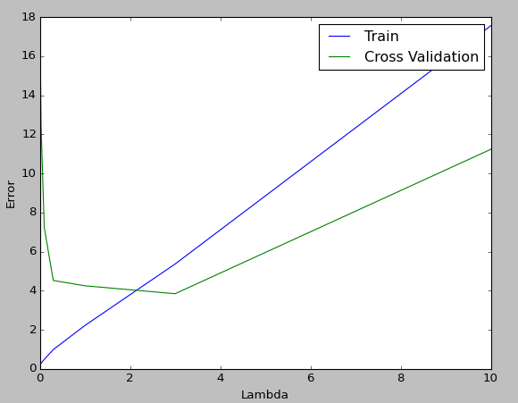
The $ \ lambda $ in the numerator of the second term is the parameter that adjusts the strength of regularization. As we saw above, this corresponds to the ʻalpha parameter in linear_model.Ridge () `. As with Coursera, change this parameter to 0.001, 0.003, 0.01, 0.03, 0.1, 0.3, 1, 3, 10 and plot the learning curve to see which $ \ lambda $ is right for you.

Click here for the code.

#Calculate the factorial of X and create a new feature X_Let it be poly
#X is the m x 1 matrix, X_poly is an m x 8 matrix
poly = preprocessing.PolynomialFeatures(degree=8, include_bias=False)
X_poly = poly.fit_transform(X) #Training data
Xval_poly = poly.fit_transform(Xval) #Cross Validation data

#Try drawing a Learning Curve by changing λ
error_train = np.zeros(9)
error_val = np.zeros(9)
lambda_values = np.array([0.001, 0.003, 0.01, 0.03, 0.1, 0.3, 1.0, 3.0, 10.0])
for i in range(0,9):
    # X_Linear regression using poly
    model = linear_model.Ridge(alpha=lambda_values[i]/10, normalize=True ) #Change the regularization parameter alpha
    model.fit(X_poly,y)
    #Calculate errors in training data (with regularization term)
    error_train[i] = sum( (y - model.predict(X_poly))**2 ) / (2*y.size) + sum(sum( model.coef_**2 )) * lambda_values[i]/(2*y.size)
    #Calculate errors in cross-validation data (with regularization term)
    error_val[i] = sum( (yval - model.predict(Xval_poly) )**2 ) / (2*yval.size) + sum(sum( model.coef_**2 ))* lambda_values[i]/(2*yval.size)

px = lambda_values
plt.plot(px, error_train, label="Train")
plt.plot(px, error_val, label="Cross Validation")
plt.xlabel("Lambda")
plt.ylabel("Error")
plt.legend()
plt.show()

The plot looks like this, and the result is that $ \ lambda = 3 $, which has the smallest error value in cross-validation, is good.

in conclusion

sklearn.linear_model.Ridge () also has a model called sklearn.linear_model.RidgeCV () for cross-validation, and it seems that it will calculate the optimum ʻalpha` number together when trained.

References

-Explanation of scikit-learn -Effect of L1 regularization and L2 regularization in regression model