[PYTHON] [Computer vision] Epipolar geometry to learn with cats

Introduction
The cat is cute ~
In this article, we will learn together with cats about the technology for restoring the 3D world from multi-view images, which is dealt with in the field of computer vision.
This field is still under research, and some difficult mathematical formulas come out, which sometimes makes it difficult, but I hope that the pain will be neutralized by learning with cats.
This article corresponds to Chapter 5, "5.1 Epipolar Geometry, 5.2 Calculations Using Cameras and 3D Structures" in "Practical Computer Vision". To do.
I want to restore the 3D world from a multi-view image
The image of the cat at the beginning was a two-dimensional image. So how do you restore the 3D shape of this cat?
The correct answer is ** to shoot from multiple perspectives while moving the camera towards the cat **.
Based on how the cat looks from each viewpoint, the change in the posture of the camera and the geometric structure of the cat being photographed by the camera are calculated in reverse.
This is called Structure from Motion (SfM).

The procedure is as follows.
-
** 1. Find a corresponding point ** Corresponding points are, for example, a pair of points that appear in each image when the cat's hand is viewed from different perspectives. Finding the corresponding points in the image before and after moving the viewpoint gives you a clue as to how you moved.
-
** 2. Estimate camera motion ** Estimate how the viewpoint has moved, using the corresponding points as clues.
-
** 3. Reconstruct the 3D scene ** The 3D shape is restored based on the corresponding points and the camera movement estimation result.
-
** 4. Overall optimization ** By repeating steps 2 and 3 each time the camera is moved, camera movement / 3D scene restoration errors will accumulate. In order to solve this, the overall accuracy is improved by finding the optimum solution that minimizes the error between the measured value and the estimated value using all the corresponding points and the estimation results of the viewpoint motion.
To simplify the problem, consider image pairs here. In other words, consider only two viewpoints.
First, I will explain the basic theory that occurs between these images. After that, we will estimate the camera motion and reconstruct the 3D scene. The overall optimization of 4. is a process that is necessary only when there are many viewpoints, so we will not consider it here.
Epipolar geometry is what?
Before moving the camera or restoring a 3D scene from a two-view image, it is necessary to understand the basic theory of epipolar geometry. Epipolar geometry is the geometry that occurs when you shoot the same 3D object from different perspectives with two cameras **.
The elements that systematize epipolar geometry are the epipolar plane, epipolar lines, epipoles, elementary matrices, and elementary matrices, which we will introduce next.
Five super important words that appear in epipolar geometry
-
** Epipolar plane ** (blue plane in the figure) When the optical centers of the two cameras are $ O_ {1} $, $ O_ {2} $, the three-dimensional points $ X $, $ O_ {1} $, $ O_ {2} $, a total of three points The plane through which it passes is called the epipolar plane. The blue plane in the figure.
-
** Epipolar line ** (yellow line in the figure) An epipolar line is a line where the epipolar plane and each image plane intersect. For example, when a 3D point X appears as a point x1 on image 1, it shows that the same point X appears somewhere on the epipolar line on image 2.
-
** Epipole ** (red dot in the figure) The epipolar lines of all images always intersect at one point. That is Epipole. Therefore, all epipolar lines pass through epipoles. This point is the projection of the camera center of the other image onto your image.

Corresponding points and epipolar lines drawn on the actual image:

-
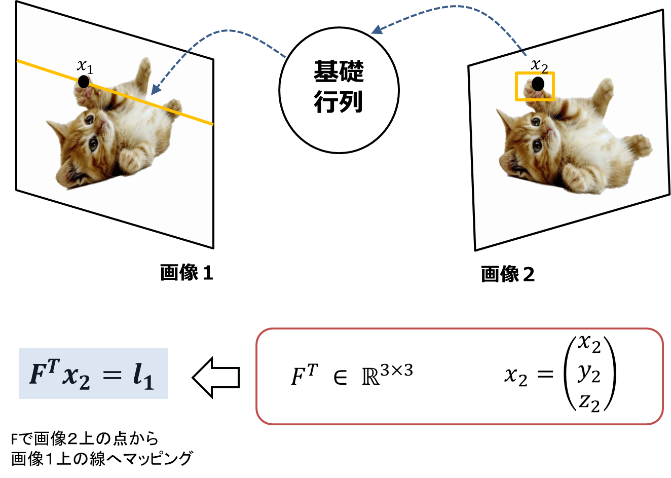
** Fundamental Matrix ** It is a 3x3 matrix and contains ** camera internal / external matrix information. ** It also has the role of ** mapping a point (0D) on one image to an epipolar line (1D) on another image. If this matrix can be estimated, it can be used later when estimating camera motion, etc., so it is very important to find this matrix correctly. Let's take a closer look next.
-
** Essential Matrix ** It has a similar name to the base matrix, but is a relative of the base matrix. A 3x3 matrix that contains ** camera external matrix information. ** You can convert $ F $ to $ E = K_ {2} FK_ {1} $ using the camera internal matrix $ K $.
Basic matrix F
Introducing the Epipolar Restraint Ceremony
If $ x_ {1} $ and $ x_ {2} $ are correspondence points, the following relationship holds for all correspondence points $ x_ {1} $, $ x_ {2} $.
\boldsymbol{x_{2}^{T}}F\boldsymbol{x_{1}} = 0
$ F $ is called the base matrix and is a 3x3 matrix. $ x_ {1} $, $ x_ {2} $ are 3D vectors that represent the coordinates of the corresponding points in the ** image coordinate system in the simultaneous coordinate system.
This formula shows that there is a constraint relationship between the corresponding points of the two images. ** This formula is called the epipolar restraint formula. ** Once the viewpoint is decided, it will be decided (= constraint) on which side in image 2 the corresponding point found in image 1 is located. And this constraint formula depends only on ** two viewpoints and not on the 3D scene at all. ** **

Now, let's check if $ \ boldsymbol {x_ {2} ^ {T}} F \ boldsymbol {x_ {1}} = 0 $ holds.
Since $ x_ {1} $ is a point on image 1, it is expressed as $ x_ {1} = (x_ {1}, y_ {1}, z_ {1}) ^ {T} $ ($ z_ {1) } $ Is 1).
On the other hand, since F is a 3x3 matrix, $ Fx_ {1} $, which is the product of $ x_ {1} $, is a 3D vector. Let this vector be $ Fx_ {1} = (a, b, c) ^ T $.
This $ Fx_ {1} = (a, b, c) ^ T $ is the coefficient of the epipolar line on image 2. And when this coefficient is multiplied by x2 on the epipolar line, it shows that the linear equation $ ax + by + c = 0 $ is satisfied. In other words, $ \ boldsymbol {x_ {2} ^ {T}} F \ boldsymbol {x_ {1}} = 0 $ holds!
Conversely, if the result of substituting $ x_ {2} $ is non-zero, then that point $ x_ {2} $ is not the corresponding point of x1 (see figure below).

When searching for the corresponding point $ x_ {2} $ in image 2 of the point $ x_ {1} $ in image 1, instead of searching for the entire image in ** image 2, $ x_ {1} $ Only the epipolar line $ l_ {2} $ projected on image 2 needs to be searched **, so the calculation cost and error response rate will decrease.
By the way, the above equation $ \ boldsymbol {x_ {2} ^ {T}} F \ boldsymbol {x_ {1}} = 0 $ maps the point $ x_ {1} $ on image 1 to image 2 as a straight line. It represents the case. On the contrary, when the point $ x_ {2} $ on the image 2 is mapped to the image 1 as a straight line, the following equation is obtained, and both sides are transposed, so it is mathematically the same. ($ (\ Boldsymbol {x_ {2} ^ {T}} F \ boldsymbol {x_ {1}}) ^ {T} = $ The following formula)
\boldsymbol{x_{1}^{T}}F^{T}\boldsymbol{x_{2}} = 0
The point is that the positions of $ x_ {1} $ and $ x_ {2} $ are swapped and F is transposed.
1. Find F
So how do you find F? There are several typical methods for that.
-
** 8-point algorithm ** Estimate F using 8 or more corresponding points. Solve with least squares using SVD. For practical use, use the normalized 8-point algorithm.
-
** Normalized 8-point algorithm ** An improved version of the 8-point algorithm. As a normalization process, the origin is moved to the center of gravity of the point cloud of the corresponding points, and the average distance from the center of gravity to each corresponding point is set to $ \ sqrt2 $, so that the accuracy is significantly improved. [Normalization 8-point algorithm implementation] (http://www.peterkovesi.com/matlabfns/Projective/fundmatrix.m) Normalization implementation
-
** Algebraic cost minimization (repetition) ** It is more accurate than the normalized 8-point algorithm.
-
** Minimize the error in the distance between the observation point and the estimation point ** After giving F as the initial value by the above method, calculate the position of X once and project it on the image. The distance (error) between the observation point and the estimation point is minimized as a cost function. It is called the Gold Standard Algorithm and has the highest accuracy.
Also, if you know the two camera matrices, you can also find them Implementation
8-point algorithm
Here is an overview of the most basic 8-point algorithm (see the link above for a detailed implementation).
The epipolar constraint expression $ \ boldsymbol {x_ {2} ^ {T}} F \ boldsymbol {x_ {1}} = 0 $ gives one equation below for each correspondence point i.

Since the unknown variable is an F matrix here, we will summarize F and solve it for f in the form of the equation Af = 0. Here, F is a 3x3 matrix, but since the scale is indefinite, it can be solved if there are practically 8 corresponding points. The name of the "8-point algorithm" comes from here.

After disassembling with SVD, use that F is rank 2. If the minimum singular value of the diagonal component of Σ is set to 0 and solved, the accuracy of F will increase. The left side of the figure below is the case where the constraint of rank 2 is not applied, and the right side is the case where the constraint of rank 2 is applied.
 Quoted from reference [1].
2. Find the camera matrix from F
So why did we find F? Because we can find the camera matrix P from ** F **.
As mentioned earlier, F contains an internal camera matrix and an external camera matrix. Therefore, if F is decomposed into internal and external camera matrices, the camera matrix can be estimated from F.
However, the accuracy of the estimation depends on whether or not the camera has been calibrated in advance. If the internal parameters of the camera are unknown, only the projective transformation can be estimated from F.
The process flow from F to estimating the camera matrix is as shown in the figure below.

If the camera is not calibrated
If the camera is not calibrated, that is, if the camera's internal parameters are unknown, then both the camera's internal and external parameters must be estimated. In this case, ** the camera matrix can only be estimated up to the projective transformation. ** **
Normally, P to F can be calculated as one, but ** the opposite, F to P cannot be calculated as one **. This is because the basic matrices of the two sets of projected images are the same.
For example, the F of the camera matrix (P, P'H) and the F of the camera matrix (PH, P'H) are the same.
The camera matrix $ P_ {1} $, $ P_ {2} $ is as follows. × is the outer product.
P_{1}=[I|0]And P_{2} =[[e_{2}]×F|e_{2}]
If the camera has been calibrated
If the camera has been calibrated, you only need to estimate the camera external parameters. All parameters can be estimated except for the translational scale. F has the ambiguity of projective transformation, while E has the ambiguity of having four solutions.
First, find the base matrix E from F using $ E = K_ {2} FK_ {1} $. Next, E is decomposed by SVD. Since E has det (E) = 0 and the non-zero singular values are equal and their magnitudes are indefinite, the diagonal component of Σ can be written as (1,1,0). In other words, it can be decomposed by SVD as follows.
E=Udiag(1,1,0)V^{T}
$ u_ {3} $ is the vector of the third column of $ U $
W = \begin{pmatrix}
0 & -1 & 0 \\
1 & 0 & 0 \\
0 & 0 & 1
\end{pmatrix}
Then, in the end, the camera matrix has the following four solutions.

Of these, only one has the scene in front of the camera, so (a) is the correct solution. (Figure below)

Quoted from reference [1].
3. Rebuild the 3D world
The camera matrix P has been obtained. Let's finally reconstruct the three-dimensional world.
Triangulation
Triangulation estimates X that simultaneously satisfies the following camera conversion formulas obtained from two viewpoints.

Quoted from reference [1].
From the camera conversion formula where the camera matrix is $ P_ {1} $, $ P_ {2} $
\lambda_{1}x_{1} = P_{1}X
\lambda_{2}x_{2} = P_{2}X
So, if you express it in a matrix,
\begin{bmatrix}
P_{1} & -x_{1} & 0 \\
P_{2} & 0 & -x_{2}
\end{bmatrix}
\begin{bmatrix}
X \\
\lambda_{1}\\
\lambda_{2}
\end{bmatrix}
=0
It will be.
Since this is also in the form of Ax = 0, 3D X can be restored by solving x with SVD.
Implementation
- ykoga/cv_tutorial_epipolar (OpenCV)
- From OpenCV3.1 (released 12/12/2015), sfm module with Structure From Motion function has been added.
Reference material
- Books
[1] Multiple View Geometry in Computer Vision
[2] Practical Computer Vision - Implementation MATLAB and Octave Functions for Computer Vision and Image Processing
- Image Pakutaso GATAG | Free Image / Photograph Collection 3.0
- Other Fundamental Matrix Song
Recommended Posts