Image processing by matrix Basics & Table of Contents-Reinventor of Python image processing-
A story about image processing only by matrix operation without relying on the image processing library. Also possible with Pythonista
Intermediate editions Drawing ・ Grayscale ・ [Convolution filtering](http: // qiita.com/secang0/items/f3a3ff629988dc660d87) ・ Affine transformation
Preface
What is a "reinventor"?
Instead of relying on Open CV or Pillow, I will actually write various image processing using numpy and matplotlib. It's a combination that can also be used with the iOS app Pythonista.
Execution environment
In addition to the standard library, use numpy and matplotlib. I don't use pandas or scipy. This combination seems to be a grammar that is easy for matlab users to use.
Python 3 on Windows 10.5.2|Anaconda 4.2.0 numpy 1.12.1|matplotlib 2.0.0 Numpy 1.8.0 | matplotlib 1.4.0 in Pythonista3 I have confirmed the operation with.
import numpy as np
import matplotlib.pyplot as plt
Prerequisite knowledge
It assumes knowledge of python 3 and knowledge of numpy and matplotlib. (The rest is attached with numpy, such as matrix knowledge)
Basics
Load / display / save images
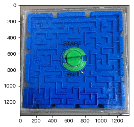
Use matplotlib.pyplot to load, display and save images. Also, the read image is stored in numpy.ndarray. This time, let's read and write labyrinth.jpeg in the same directory.

#Loading images
#3D np in img.The array of array is stored.
img = plt.imread('labyrinth.jpeg')
type(img) #=> numpy.ndarray
img.size #=> (1367, 1345, 3)


#Image display
plt.imshow(img)
plt.show() #When the image used is small, it looks blurry, but don't worry about it now

#Save image
plt.imsave('labyrinth-1.jpeg', img) #Extension.Even if you change it to png, it will be saved properly.
Please be assured that the horizontal scale is not available when you save it.
It is no exaggeration to say that we now have input, output and debugging tools.
Pixel homebrew
Some people may want to create an image by specifying the pixels themselves. In such a case, you can specify the pixels with a 2D or 3D np.array, but here is a little trick, so I will introduce it.
Black-and-white image (two-dimensional array of (height = 3) * (width = 3))
img_gray = np.array([
                    [0,63,127],
                    [63,127,0],
                    [255,0,127]
], dtype = np.uint8)

#Image display
plt.imshow(img_gray, cmap = 'gray', vmin = 0, vmax = 255, interpolation = 'none')
plt.show()

First of all, a black and white image. There are about four places I don't understand.
dtype = np.uint8cmap = 'gray'vmin = 0, vmax = 255interpolation = 'none'
Is.
Let's explain each. (1 and 3 will be explained together)
dtype = np.uint8, vmin = 0, vmax = 255 If you've used a color picker, you'll find that colors are often represented between 0 and 255. However, that trick is needed to convey this to plt.
The dtype specification is actually unnecessary this time. Rather, this is a useful designation for color, but it seems to be worth it. For black and white images, it is necessary to specify vmin and vmax. If this is omitted, it will be normalized by imshow () without permission.
cmap = 'gray' Given that cmap stands for colormap and gray means gray, it's pretty predictable. In other words, it is a specification to interpret one-dimensional data as black-gray-white. If you try this and change it to one of in this, the interpretation will change and the color will change. (For example, using YlOrBr_r is sepia-like) Create your own cmap It is also possible.
interpolation = 'none' This removes the filter that is applied on its own. (Rather, antialiasing) I don't know why it's applied from the beginning, but at least it's annoying to make sure each pixel is the color you want, so I'll remove it. Maybe this depends on the version.
RGB image ((height = 3) * (width = 3) * (RGB) three-dimensional array)
img_rgb = np.array([
                    [[255,0,0],[0,255,0],[0,0,255]],
                    [[255,255,0],[0,255,255],[255,0,255]],
                    [[0,0,0],[127,127,127],[255,255,255]],
], dtype = np.uint8)

#Image display
plt.imshow(img_rgb, cmap = 'gray', vmin = 0, vmax = 255, interpolation = 'none')
# => plt.imshow(img_rgb, interpolation = 'none')Same as

plt.show()

The code is almost the same as before. (Even if you specify cmap, vmax, vmin, it will be ignored)
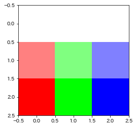
RGBA image ((height = 3) * (width = 3) * (RGBA) three-dimensional array)
img_rgba = np.array([
                    [[255,0,0,0],[0,255,0,0],[0,0,255,0]],
                    [[255,0,0,127],[0,255,0,127],[0,0,255,127]],
                    [[255,0,0,255],[0,255,0,255],[0,0,255,255]],
], dtype = np.uint8)

#Image display
plt.imshow(img_rgba, cmap = 'gray', vmin = 0, vmax = 255, interpolation = 'none')
# => plt.imshow(img_rgba, interpolation = 'none')Same as

plt.show()
Similarly, the code is almost the same as before.
As a reminder, A in RGBA is an alpha A for transparency. It's hard to tell if this is transparent even if you look at the image above, but if you look at it with gimp etc., you can see that it is transparent.
 (Image superimposed on the checkered pattern)
For the time being, create a function that summarizes these.
def img_show(img : np.ndarray, cmap = 'gray', vmin = 0, vmax = 255, interpolation = 'none') -> None:
    '''np.Display an image with array as an argument.'''

    #Set dtype to uint8
    #Overflow and underflow handling

    img = np.clip(img,vmin,vmax).astype(np.uint8)

    #Display image
    plt.imshow(img, cmap = cmap, vmin = vmin, vmax = vmax, interpolation = interpolation)
    plt.show()
    plt.close()
Now you can make your own pixel art.
Enlargement (simple enlargement)
The enlargement dealt with here is an integer multiple and an enlargement without interpolation. Use repeat.
#Magnified 5 in the vertical direction and 3 times in the horizontal direction
#Loading images
img = plt.imread('labyrinth.jpeg')

#Enlarge image
img_expand = img.repeat(5, axis = 0).repeat(3, axis = 1)

img_show(img_expand)
 At first glance, it shrinks in the horizontal direction, but if you look at the scale, it is enlarged. (You may check with img_expand.size)
This is an extension that is rarely used, and the expansion that is actually used will be described later. (plans)
Arrange images
Try arranging the same images horizontally or vertically. concatenate is convenient.
img = plt.imread('labyrinth.jpeg')

img_verticle = np.concatenate((img, img), axis = 0) #Vertical
img_horizontal = np.concatenate((img,)*3, axis = 1) #side

#Image display
img_show(img_verticle)
img_show(img_horizontal)


In the horizontal image, the number of repetitions is specified by multiplying the tuple.
Trimming to a quadrangle (3/30 added)
Trimming can be done easily by index operation.
img = plt.imread('labyrinth.jpeg')

#1000 vertically:1500, 0 beside:Cut out 500
img_show(img[1000:1500,0:500])

RGB decomposition
def decomposition(img : np.ndarray, channel : list = [1.,1.,1.]) -> np.ndarray:
    '''Emphasize each channel with the intensity given to the channel'''

    float_img = img * channel
    return np.array(float_img,dtype = np.uint8)

img = plt.imread('labyrinth.jpeg')
img_show(decomposition(img, [1.,0.,0.]), cmap = 'Reds')
img_show(decomposition(img, [0.,1.,0.]), cmap = 'Greens')
img_show(decomposition(img, [0.,0.,1.]), cmap = 'Blues')


 The above code defines a function called decomposition (channel decomposition seems to be called color decomposition in English). This is basically an operation of ʻimg * [0,0,1] `, but since the type is a little complicated, I defined a function.
I checked it with gimp just in case, but it looked the same.
Grayscale

Converting a pixel with three-dimensional RGB values to a pixel with only one-dimensional Y values is called grayscale. In short, it is a method of creating a black and white image. There are various grayscale methods, but here we only deal with the median method and the G-channel method.
Median method
The median method uses the average of the maximum value in RGB and the minimum value in RGB as Y.
In other words, a calculation like (max (R, G, B) + min (R, G, B)) / 2 is performed.
img = plt.imread('labyrinth.jpeg')

img_mid_v = np.max(img, axis = 2)/2 +np.min(img, axis = 2)/2
img_show(img_mid_v)

Here, one point. About the calculation formula of img_mid_v ʻImg_mid_v = (np.max (img, axis = 2) + np.min (img, axis = 2)) / 2` may raise the question. The answer is "No." The reason is that if you add the maximum and minimum values first, uint8 will overflow. After the type becomes float, it returns to uint8 with img_show.
By the way, np.max (img, axis = 2) // 2 + np.min (img, axis = 2) // 2 does not change much, but the minimum and maximum values are truncated respectively. I want to be careful.
G channel
It seems that humans recognize G most strongly among RGB. The G-channel method paid attention to this. In the G channel method, the value of G is regarded as the value of Y. In short, it's a very rough method, but it's reasonably effective, so humans are strange. (It is even more strange that there should be as many pyramidal cells as R and G on the retina)
The code is simple. ... is called Ellipsis This is a convenient symbol.
img = plt.imread('labyrinth.jpeg')
img_g_channel = img[...,1]
img_show(img_g_channel)

The idea is the same as the previous RGB decomposition. However, it is regrettable that it will not be long before this simple method is applied.
Other methods will be dealt with in the future.
Binarization
Now that you have a black and white image, try binarization, where the Y value is "1 for pixels above the threshold and 0 for pixels below the threshold". For black and white images, use the one created by the G channel method.
img = plt.imread('labyrinth.jpeg')
img_g_channel = img[...,1]

#Threshold setting
threshold = 75

img_binary = img_g_channel >= threshold
img_binary = np.uint8(img_binary * 255)
img_show(img_binary)

Somehow, I feel that the maze is emerging.
Convolution filter
At the end of the basics, I will introduce how to make a filter by convolution. Spatial filtering is easy to understand for the filter by convolution.
The filter used this time uses the following two matrix convolutions.
\frac{1}{256}\left(
\begin{matrix}
21 & 31 & 21 \\
31 & 48 & 31 \\
21 & 31 & 21
\end{matrix}
\right)
This is a blur filter, often called Gaussian blur. This is a filter often used for denoising prior to contour extraction.
\left(
\begin{matrix}
0 & -1 & 0 \\
-1 & 4 & -1 \\
0 & -1 & 0
\end{matrix}
\right)
This is a Laplacian filter and is often used for contour extraction. Can a person who can easily understand the expression that the idea is the same as the on center bipolar cell have reached this point?
First, create a function to convolve a 2D array (you don't have to create it yourself using scipy or PIL, but unfortunately you have to create it yourself under the binding conditions of Numpy and matplotlib.
def convolve2d(img, kernel):
    #Calculate the size of the submatrix
    sub_shape = tuple(np.subtract(img.shape, kernel.shape) + 1)

    #Since the function name is long, it is omitted once
    strd = np.lib.stride_tricks.as_strided

    #Create a matrix of submatrix
    submatrices = strd(img,kernel.shape + sub_shape,img.strides * 2)

    #Calculate the Einstein sum of the submatrix and the kernel
    convolved_matrix = np.einsum('ij,ijkl->kl', kernel, submatrices)

    return convolved_matrix
The above code convolves using the matrix of the img submatrix. See stackoverflow teacher for more information.
#Creating a filter kernel
gaussian = np.array([[21,31,21],
                     [31, 48,31],
                     [21,31,21]])/256
laplacian = np.array([[ 0,-1, 0],
                      [-1, 4,-1],
                      [ 0,-1, 0]])

#Loading images
img = plt.imread('labyrinth.jpeg')
img = img[...,1] #This time, only the G channel is targeted.

#Apply Gaussian blur 20 times
for _ in range(20):
    img = convolve2d(img, gaussian)

At this point, it may seem like a cut-off change, but if you save it in bmp and enlarge it, you will find that it is surprisingly different.

#Apply Laplacian filter
img = convolve2d(img, laplacian)
plt.imshow(b,cmap = 'gray_r', vmax = img.max()*0.5)
#The maximum value is not always 255.
#Also, when adjusted to the maximum value, other values were crushed, so*0.Corrected by 5.

plt.show()
plt.close()

It's a little lacking in impact, so let's summarize the basics.
img = np.array([
                [[  0,  0,  0],[  0, 63,127],[255,  0,  0]],
                [[ 63, 63, 63],[  0,  0,255],[  0,  0,  0]],
                [[255,255,255],[  0,  0,  0],[ 63,127,  0]]
], dtype = np.uint8)


img = img.repeat(100,axis = 1).repeat(100,axis = 0)#Expansion
img = np.concatenate((img,)*2, axis = 1) #Copy horizontally
img = np.concatenate((img,)*2, axis = 0) #Copy vertically
print('RGB image')
img_show(img)


#Generate black and white images using the median method
img = np.array(np.max(img, axis = 2)/2 +np.min(img, axis = 2)/2, dtype = np.uint8)
print('Black and white image')
img_show(img)

#Gaussian blur
img = convolve2d(img, gaussian)

#Contour extraction
img = convolve2d(img, laplacian)

print('Contour extraction')
plt.imshow(img,cmap = 'gray_r', vmax = img.max())
plt.show()
plt.close()
RGB image
 Black and white image
 Contour extraction

In the basic edition, we also saw the G-channel method and binarization.
Intermediate
** * We will add it little by little, so if you are interested, please keep it in stock. ** ** It's already too long, so I've kept it in the outline and table of contents. For more information, please follow the link. Also, the images used will change from the intermediate edition. Why did I use an image without red ...
Drawing of figures (added on 3/30 days)
To draw a figure, use msgid to get the coordinates on the image.
x, y = np.mgrid[:100,:100]
Note that the positive direction of $ x $ is down and the positive direction of $ y $ is right.
** For those who want to learn more **
Grayscale (added on 3/30)
Grayscale is a method of calculating the black and white value Y from the RGB values assigned to each pixel. Here, various grayscale methods that were not dealt with in Basics ) Also try. See the link for a detailed explanation. They are treated in the same order.
** For those who want to learn more **
Convolution filtering (added 4/1)
Handles low-pass filters, high-pass filters, and differential filters.
** For those who want to learn more **
Affine transformation (added 4/5 days)
There are many ways to distort an image. A transformation that combines linear transformation (scaling, rotation, shearing) and translation is called affine transformation. ** For those who want to learn more **
Recommended Posts