[PYTHON] Introduction to Monte Carlo Method
Introduction
Nowadays, the Bayesian approach is no longer the norm, and how to collect learning data and dive into deep learning is popular, but sometimes you may do such classical calculations.
I intended to explain MCMC, but it was not easy to explain simple simulation, so I will explain simple simulation once. I personally want to write about MCMC in the near future.
This article is largely based on Chapter 11 of PRML.
Monte Carlo method
When you're involved in machine learning, you'll often hear the word Monte Carlo simulation, or the Monte Carlo method. Before I wrote this article, I was vaguely thinking, "Ah, MCMC, right?", But when I tried to explain it concretely, I got stuck in the answer. In such a case, if you ask Wikipedia, you can understand the general idea, so I would like to take a look at the Wikipedia article for the time being.
Monte Carlo method (Monte Carlo method, (English):Monte Carlo method (MC) is a general term for methods that perform simulations and numerical calculations using random numbers.
Named after Monte Carlo, one of the four districts (Cartier) of the Principality of Monaco, famous for its casinos.
Monte Carlo was just a place name. When I heard the word casino, I wondered if the people who were trying to win at the casino created it to do a simulation.
In the field of theory of computation, the Monte Carlo method is defined as a randomized algorithm that gives an upper bound on the probability of making a mistake.[1]。
In other words, most things can be called Monte Carlo simulation or Monte Carlo method by using random numbers. In fact, the article states that the "Miller-Rabin Primality Test", an algorithm that stochastically determines whether or not a prime number is a prime number, is also the Monte Carlo method. However, this time I'm focusing on machine learning, and I have no time to overlook the primality test method.
Therefore, I would like to limit my thinking to the following.
Consider an algorithm that generates a random number X that follows the distribution of P when a certain probability distribution P is determined.
If you can generate the random number $ X $ that appears in the above problem setting, you can apply it to various simulations and numerical calculations.
table of contents
--Change of variables --Exponential distribution
- normal distribution --Cauchy distribution --Rejection sampling method --Gamma distribution
Suppose it is possible to generate a uniformly distributed random number $ U $ of $ [0, 1] $ throughout. From this $ U $, a random number that follows the famous probability distribution
Change of variables
Let $ P $ be the probability distribution you want to generate.
A variable transformation method for finding a function $ F_ {P} $ such that "$ Y = F_ {P} (U) $ follows the distribution of $ P $" for a uniformly distributed random number $ U
Since $ u and y $ are appearing at the same time, it makes me feel like I don't understand. However, since there is a relation of $ Y = F_ {P} (U) $, using the inverse function $ F_ {p} ^ {-1} $ of $ F_ {p} $, $ U = F_ {p You can write} ^ {-1} (Y) $. Using this formula, we can see that we can write $ p (y) = du / dy = d (F_ {p} ^ {-1} (y)) / dy $. In fact, I think this formula transformation is pretty tricky. It's hard to understand, at least at first glance. You may be wondering why the inverse function appears, but let's get used to it little by little by looking at the example below.
Example: Exponential distribution
The probability density function $ p $ of the exponential distribution is expressed by the following formula.
Set $ G (x) = \ int_ {0} ^ {x} p (x) dx $. When the integrated function is differentiated, it returns to the original function, so $ dG / dx = p (x) $ holds. I wanted to find a function that satisfies $ p (y) = d (F_ {p} ^ {-1} (y)) / dy $, so I feel that the inverse function of $ G $ is $ F $. (Actually so).
If you calculate $ G $ concretely,
import numpy as np
import matplotlib.pyplot as plt

Lambda = 0.1
N = 100000
u = np.random.rand(N)
y = - Lambda * np.log(1 - u)

plt.hist(y, bins=200)
plt.show()
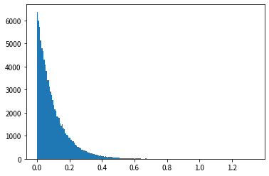
Looking at the results of the histogram, we can see that the shape is similar to the probability density function of the exponential distribution, and that random numbers that follow the exponential distribution can be generated.
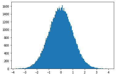
Example: normal distribution
Next, I will introduce the "Box-Muller algorithm", which is a famous algorithm for creating random numbers with a standard normal distribution. From uniform distribution $ (z_1, z_2) $ on a disk with radius 1
I gave the formula in an amakudari manner because I gave up deriving this formula. ..
I actually wrote a Python script that generates random numbers using this function $ F $.
import numpy as np
import matplotlib.pyplot as plt

N = 100000
z = np.random.rand(N * 2, 2) * 2 - 1
z = z[z[:, 0] ** 2 + z[:, 1] ** 2 < 1]

z = z[:N]
r = z[:, 0] ** 2 + z[:, 1] ** 2
y = z[:, 0] / (r ** 0.5) * ((-2 * np.log(r)) ** 0.5)

plt.hist(y, bins=200)
plt.show()
Cauchy distribution
Finally, let's generate a random number that follows the Cauchy distribution. The Cauchy distribution is rarely used statistically when compared to the exponential and normal distributions. However, in the next section, the gamma distribution section uses random numbers that follow the Cauchy distribution, so we will introduce them here. The probability density function of the Cauchy distribution is expressed by the following formula.
p(x; c) = \frac{1}{1 + (x - c)^2}
The cumulative distribution function $ G $ of the Cauchy distribution can be easily written as follows by using the inverse function of the $ \ tan $ function called $ \ arctan $.
u = G(x) = \int_{-\infty}^{x} p(x; c) = \frac{1}{\pi} \arctan (x - c) + \frac{1}{2}
Therefore, the inverse function $ F $ of $ G $ can be written as follows.
F(u) = \tan \bigg(\pi \bigg(u - \frac{1}{2} \bigg)\bigg) + c
That is,
Let's see the result of actually generating random numbers using this function $ F $.
cauchy_F = lambda x: np.tan(x * (np.pi / 2 + np.arctan(c)) - np.arctan(c)) + c

N = 100000
u = np.random.rand(N)
y = cauchy_F(u)
y = y[y < 10]

plt.hist(y[y < 10], bins=200)
plt.show()
Looking at the results of the histogram, we can see that the shape is similar to the probability density function of the exponential distribution, and that random numbers that follow the exponential distribution can be generated.
However, if you take a closer look at the script, you'll find a line that looks like y = y [y <10].
If you remove this line and execute it, it will be ridiculous.
This means that ridiculously large outliers can be generated. This result is somewhat convincing, recalling the fact that the mean Cauchy distribution diverges.
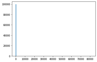
If I limit the random number value to 10 or less, I think that the average value is around 2, but since an extremely large value rarely occurs, the average value has been pushed upward. I remember the story of the difference between the average income and the median income.
Points of change of variables
You need to be familiar with the characteristics of the distribution. In most cases, you need to be able to write the cumulative distribution function in a simple form. I think it would be a lot of work to ask for it in any other way. Also, if F is not a function that can be easily calculated, it makes no sense after all.
Rejection sampling method
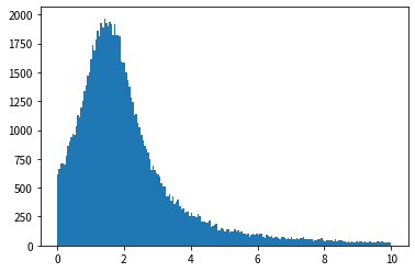
Example: gamma distribution
The probability density function of the gamma distribution is expressed by the following formula.
p(x; a, b) = b^{a} z^{a-1} \exp(-bz) / \Gamma(a)
Finding the value of the $ \ Gamma $ function is difficult, so use $ \ tilde {p} $, ignoring the $ \ Gamma $ part.
\tilde{p}(x; a) = z^{a-1} \exp(-z)
Now let's find k that exceeds the Cauchy distribution. It was troublesome to calculate by hand, so I relied on the script this time.
gamma_p_tilda = lambda x: (x ** (a - 1)) * np.exp(-x)
cauchy_p = lambda x: 1 / (1 + ((x - c) ** 2)) / (np.pi / 2 + np.arctan(c))

z = np.arange(0, 100, 0.01)
gammas = gamma_p_tilda(z)
cauchys = cauchy_p(z)

k = np.max(gammas / cauchys)
cauchys *= k

plt.plot(z, gammas, label='gamma')
plt.plot(z, cauchys, label='cauchy')

plt.legend()

plt.show()
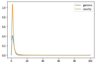
The value of $ k $ stored in the above script was $ 2.732761944808582 $.
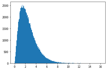
N = 100000
u = np.random.rand(N * 3)
y = cauchy_F(u)

u0 = np.random.rand(N * 3)

u0 *= k * cauchy_p(y)

y = y[u0 < gamma_p_tilda(y)]
y = y[:N]

plt.hist(y, bins=200)
plt.show()
Applicable conditions for rejection sampling
We need to have a proposed distribution $ Q $ that can easily generate random numbers. You also have to calculate $ k $ that satisfies $ kq \ geq p $. If the value of $ k $ is inadvertently increased too much, the random numbers generated must be rejected, so we want to make $ k $ as small as possible. However, in that case, it is necessary to derive from the concrete form of the function or calculate the value precisely, which is a decent amount of trouble. Also, when determining the value of $ k $ or calculating whether to reject it, the value of the probability density function is used for both $ P $ and $ Q $, so the probability density function itself must be easy to calculate. Therefore, this method cannot be applied when the calculation of the probability density function itself is difficult, such as in a model in which multiple variables are intricately intertwined.
Towards MCMC
So far, we have given an overview of standard random number generation methods. After looking through it, you can see that the original probability distribution needs to be in a form that is easy to handle to some extent.
It was found that statistically important random numbers such as normal distribution, exponential distribution, and gamma distribution can be generated from a uniform distribution. I think this alone can do a lot of things, but there are more complex models out there that use a Bayesian approach. This generation method alone does not have enough weapons to counter the complex Bayesian model.
Therefore, an algorithm called MCMC that can generate random numbers for a more complicated model comes out. Next time, I would like to explain the graphical model, which is the main area to apply MCMC, and the concrete method of MCMC.
Recommended Posts