[PYTHON] Coefficient de corrélation MIC qui peut gérer les relations non linéaires et test d'indépendance de Hilbert-Schmidt HSIC
Le coefficient de corrélation de Pearson est un indice bien connu pour mesurer l'indépendance des variables. Cependant, c'est un indice qui traite des relations linéaires (linéaires), et quand il y a une relation en forme de U telle qu'une fonction quadratique, il est jugé comme "aucune corrélation". MIC et HSIC sont connus comme des indicateurs pour traiter de telles relations non linéaires, j'ai donc essayé d'utiliser le package Python.
Tout le code ci-dessous a été testé avec Google Colaboratory.
Package Python qui calcule le coefficient d'information maximal (MIC)
Vous pouvez installer le pip comme suit:
!pip install minepy
Après l'installation, préparez-vous comme suit.
from minepy import MINE
mine = MINE()
Paquet Python qui calcule HSIC (Hilbert-Schmidt Independence Criterion)
Clonez Git comme suit:
!git clone https://github.com/amber0309/HSIC.git
Préparez-vous comme suit.
from HSIC.HSIC import hsic_gam
Fonction linéaire
Examinons d'abord la fonction linéaire.
%matplotlib inline
import matplotlib.pyplot as plt
import numpy as np

X = np.linspace(-1, 1, 51)
Y = X
plt.scatter(X, Y)

Le coefficient de corrélation de Pearson est
np.corrcoef(X, Y)[0, 1]
1.0
MIC est
mine.compute_score(X, Y)
mine.mic()
0.9999999999999998
Plus la valeur suivante est élevée, plus l'indépendance du HSSC est faible, et plus la valeur est petite, plus l'indépendance est élevée.
testStat, thresh = hsic_gam(X.reshape(len(X), 1), Y.reshape(len(Y), 1))
testStat / thresh
22.610487654066624
Ajoutons du bruit à la fonction linéaire.
import numpy as np

X = np.linspace(-1, 1, 51)
Y = X + np.random.rand(51,)
plt.scatter(X, Y)

Le coefficient de corrélation de Pearson est
np.corrcoef(X, Y)[0, 1]
0.9018483832673769
MIC est
mine.compute_score(X, Y)
mine.mic()
0.9997226475394071
HSIC
testStat, thresh = hsic_gam(X.reshape(len(X), 1), Y.reshape(len(Y), 1))
testStat / thresh
13.706487127525389
Calculons comment le coefficient de corrélation de Pearson change à mesure que la quantité de bruit augmente petit à petit.
D = []
C = []
for d in range(100):
    X = np.linspace(-1, 1, 51)
    Y = X + np.random.rand(51,) * d / 10
    D.append(d)
    C.append(np.corrcoef(X, Y)[0, 1])

plt.plot(D, C)

De même, calculons comment le MIC change lorsque la quantité de bruit augmente petit à petit.
D = []
C = []
for d in range(100):
    X = np.linspace(-1, 1, 51)
    Y = X + np.random.rand(51,) * d / 10
    D.append(d)
    mine.compute_score(X, Y)
    C.append(mine.mic())

plt.plot(D, C)
De même, calculons comment le HSIC change lorsque la quantité de bruit augmente petit à petit.
D = []
C = []
for d in range(100):
    X = np.linspace(-1, 1, 51)
    Y = X + np.random.rand(51,) * d / 10
    D.append(d)
    testStat, thresh = hsic_gam(X.reshape(len(X), 1), Y.reshape(len(Y), 1))
    C.append(testStat / thresh)

plt.plot(D, C)

fonction quadratique
Vient ensuite la fonction quadratique.
import numpy as np

X = np.linspace(-1, 1, 51)
Y = X**2
plt.scatter(X, Y)

Le coefficient de corrélation de Pearson est
np.corrcoef(X, Y)[0, 1]
-2.3862043230836297e-17
MIC est
mine.compute_score(X, Y)
mine.mic()
0.9997226475394071
HSIC
testStat, thresh = hsic_gam(X.reshape(len(X), 1), Y.reshape(len(Y), 1))
testStat / thresh
9.285886928766184
Ajoutons du bruit.
X = np.linspace(-1, 1, 51)
Y = X**2 + np.random.rand(51,)
plt.scatter(X, Y)

Le coefficient de corrélation de Pearson est
np.corrcoef(X, Y)[0, 1]
0.04693076570744622
MIC est
mine.compute_score(X, Y)
mine.mic()
0.5071787519579662
HSIC
testStat, thresh = hsic_gam(X.reshape(len(X), 1), Y.reshape(len(Y), 1))
testStat / thresh
5.247036645612692
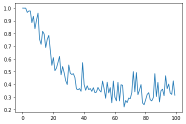
Calculons comment le coefficient de corrélation de Pearson change à mesure que la quantité de bruit augmente petit à petit.
D = []
C = []
for d in range(100):
    X = np.linspace(-1, 1, 51)
    Y = X**2 + np.random.rand(51,) * d / 10
    D.append(d)
    C.append(np.corrcoef(X, Y)[0, 1])

plt.plot(D, C)

De même, calculons comment le MIC change lorsque la quantité de bruit augmente petit à petit.
D = []
C = []
for d in range(100):
    X = np.linspace(-1, 1, 51)
    Y = X**2 + np.random.rand(51,) * d / 10
    D.append(d)
    mine.compute_score(X, Y)
    C.append(mine.mic())

plt.plot(D, C)

De même, calculons comment le HSIC change lorsque le niveau de bruit augmente petit à petit.
D = []
C = []
for d in range(100):
    X = np.linspace(-1, 1, 51)
    Y = X**2 + np.random.rand(51,) * d / 10
    D.append(d)
    testStat, thresh = hsic_gam(X.reshape(len(X), 1), Y.reshape(len(Y), 1))
    C.append(testStat / thresh)

plt.plot(D, C)

On peut voir que le coefficient de corrélation de Pearson ne pouvait pas détecter la relation de la fonction quadratique, alors que les MIC et HSIC pouvaient être détectés. Vous pouvez également voir que le MIC ne sera en grande partie pas affecté par les petits bruits.
Fonction trigonométrique
Regardons également la fonction triangulaire.
import numpy as np

X = np.linspace(-1, 1, 51)
Y = np.sin((X)*np.pi*2)
plt.scatter(X, Y)

Le coefficient de corrélation de Pearson est
np.corrcoef(X, Y)[0, 1]
-0.37651692742033543
MIC est
mine.compute_score(X, Y)
mine.mic()
0.9997226475394071
HSIC
testStat, thresh = hsic_gam(X.reshape(len(X), 1), Y.reshape(len(Y), 1))
testStat / thresh
3.212604441715373
Ajoutons du bruit.
import numpy as np

X = np.linspace(-1, 1, 51)
Y = np.sin((X+0.25)*np.pi*2) + np.random.rand(51,)
plt.scatter(X, Y)

Le coefficient de corrélation de Pearson est
np.corrcoef(X, Y)[0, 1]
0.049378342546505014
MIC est
mine.compute_score(X, Y)
mine.mic()
0.9997226475394071
HSIC
testStat, thresh = hsic_gam(X.reshape(len(X), 1), Y.reshape(len(Y), 1))
testStat / thresh
1.3135420547013614
Étudiez l'effet de l'augmentation du bruit. Le coefficient de corrélation de Pearson est
D = []
C = []
for d in range(100):
    X = np.linspace(-1, 1, 51)
    Y = np.sin((X+0.25)*np.pi*2) + np.random.rand(51,) * d / 10
    D.append(d)
    C.append(np.corrcoef(X, Y)[0, 1])

plt.plot(D, C)

MIC est
D = []
C = []
for d in range(100):
    X = np.linspace(-1, 1, 51)
    Y = np.sin((X+0.25)*np.pi*2) + np.random.rand(51,) * d / 10
    D.append(d)
    mine.compute_score(X, Y)
    C.append(mine.mic())

plt.plot(D, C)

HSIC
D = []
C = []
for d in range(100):
    X = np.linspace(-1, 1, 51)
    Y = np.sin((X+0.25)*np.pi*2) + np.random.rand(51,) * d / 10
    D.append(d)
    testStat, thresh = hsic_gam(X.reshape(len(X), 1), Y.reshape(len(Y), 1))
    C.append(testStat / thresh)

plt.plot(D, C)

On s'attendait à ce que le coefficient de corrélation de Pearson ne puisse pas détecter la relation de la fonction triangulaire avec le bruit, mais il semble que HSIC a également abandonné. Parmi eux, j'ai été surpris que MIC ait pu détecter la relation.
Fonction Sigmaid
Enfin, il y a la fonction sigmoïde.
import numpy as np

X = np.linspace(-1, 1, 51)
Y = 1 / (1 + np.exp(-X*10))
plt.scatter(X, Y)

Le coefficient de corrélation de Pearson est
np.corrcoef(X, Y)[0, 1]
0.9354020629807919
MIC est
mine.compute_score(X, Y)
mine.mic()
0.9999999999999998
HSIC
testStat, thresh = hsic_gam(X.reshape(len(X), 1), Y.reshape(len(Y), 1))
testStat / thresh
27.433932271008874
Ajoutons du bruit.
import numpy as np

X = np.linspace(-1, 1, 51)
Y = 1 / (1 + np.exp(-X*10)) + np.random.rand(51,)
plt.scatter(X, Y)

Le coefficient de corrélation de Pearson est
np.corrcoef(X, Y)[0, 1]
0.7994507640548881
MIC est
mine.compute_score(X, Y)
mine.mic()
0.9997226475394071
HSIC
testStat, thresh = hsic_gam(X.reshape(len(X), 1), Y.reshape(len(Y), 1))
testStat / thresh
12.218008194240534
Voyons l'effet de l'augmentation du bruit. Le coefficient de corrélation de Pearson est
D = []
C = []
for d in range(100):
    X = np.linspace(-1, 1, 51)
    Y = 1 / (1 + np.exp(-X*10)) + np.random.rand(51,) * d / 10
    D.append(d)
    C.append(np.corrcoef(X, Y)[0, 1])

plt.plot(D, C)

MIC est
D = []
C = []
for d in range(100):
    X = np.linspace(-1, 1, 51)
    Y = 1 / (1 + np.exp(-X*10)) + np.random.rand(51,) * d / 10
    D.append(d)
    mine.compute_score(X, Y)
    C.append(mine.mic())

plt.plot(D, C)

HSIC
D = []
C = []
for d in range(100):
    X = np.linspace(-1, 1, 51)
    Y = 1 / (1 + np.exp(-X*10)) + np.random.rand(51,) * d / 10
    D.append(d)
    testStat, thresh = hsic_gam(X.reshape(len(X), 1), Y.reshape(len(Y), 1))
    C.append(testStat / thresh)

plt.plot(D, C)

Tous les indicateurs peuvent détecter la relation, mais en termes de résistance au bruit, le MIC semble être le plus fort.
C'est une impression individuelle
MIC MIC!