[PYTHON] L'exemple de Miyashita de la mécanique analytique, des exercices résolus et déplacés avec l'animation

Miyashita Je résous des exercices de mécanique analytique. Si vous constatez des erreurs, veuillez nous en informer.

Chapitre 1

Pour les mouvements pendulaires de longueur $ l $, l'angle $ \ phi $ est la seule variable de fond. Il est plus pratique d'exprimer la position du gage en coordonnées polaires plutôt qu'en coordonnées cartésiennes. En faisant bon usage des variables qui prennent en compte les conditions de liaison de cette manière, il est possible de gérer des variables de mouvement substantielles.

Trouvez le lagrangien du pendule (Fig. 1.3) en coordonnées orthogonales (x, y). (Exemple au chapitre 2 p.11)

L'énergie cinétique est $ T = 1 / 2m \ dot {x} ^ 2 + 1 / 2m \ dot {y} ^ 2 $, et l'énergie potentielle est $ U = mgy $ Par conséquent, Lagrangean $L=\frac{m}{2}(\dot{x}^2+\dot{y}^2)-mgy$ Aussi, voici les conditions contraignantes x^2+y^2=l^2 Il y a.

Trouvez le lagrangien du pendule (Fig. 1.3) en coordonnées polaires (l, Φ). (Exemple au chapitre 2 p.12)

x=l\sin \phi y=-l\cos \phi Que \dot{x}=\dot{l}\sin \phi + l\dot{\phi}\cos \phi \dot{y}=-\dot{l}\cos \phi + l\dot{\phi}\sin \phi Donc \frac{m}{2}(\dot{x}+\dot{y})^2=(\dot{l}\sin \phi + l\dot{\phi\}cos \phi)^2+(\dot{l}\sin \phi + l\dot{\phi}\cos \phi)^2=\frac{m}{2}(\dot{l}^2+l^2 \dot{\phi}^2) U=mgl\cos \phi Parce que $ l $ est constant L=\frac{m}{2}(l^2 \dot{\phi}^2)+mgl\cos \phi Les conditions de liaison peuvent être bien gérées en coordonnées polaires.

Équation du mouvement

L'équation du mouvement de Lagrange \frac{d}{dt}\frac{\partial L}{\partial \phi}=ml^2\ddot{\phi} \frac{\partial L}{\partial \phi}=-mgl\sin \phi \therefore \ddot{\phi}=-\frac{g}{l}\sin \phi

Résolution de l'équation du mouvement

Trouvez la solution des vibrations minuscules près de Φ = 0.

Quand Taylor s'étend au premier \dot{\phi}=\frac{p_φ}{ml^2} \dot{p_\phi}=mgl\phi Sera. Donc \ddot{\phi}=-\frac{g}{l}\phi La solution générale de cette équation est \phi=A\cos(\sqrt{\frac{g}{l}}t+B) Si $ \ phi = \ phi_0 << 1, \ \ dot {\ phi} = 0 $ A=\phi_0, \ \dot{\phi}=A\frac{g}{l}\sin(B)=0 \therefore B=0 Donc, \phi=\phi_0 \cos(\sqrt{\frac{g}{l}}t)

Trouvez la solution de la vibration avec Φ0 comme valeur initiale.

\ddot{\phi_1}=-\frac{g}{l}\sin(\phi_1) Ici $ \ phi_1 = \ phi + \ phi_0 $ La solution de cette équation peut être facilement obtenue par analyse numérique de Python. Il est nécessaire de changer l'équation différentielle du second ordre en l'équation différentielle du premier ordre. \dot{\phi}=\omega \dot{\omega}=-\frac{g}{l}\sin \phi

Python utilise scipy.integrate.solve_ivp. Cela donne l'intégrale de l'équation différentielle ordinaire avec la valeur initiale.

scipy.integrate.solve_ivp(fun, t_span, y0, method='RK45', t_eval=None, dense_output=False, events=None, vectorized=False, args=None, **options) Dans

amusant: fonction t_span: plage d'intégration y0: valeur initiale méthode: 'RK45 méthode explicite runge-tack t_eval: Temps d'enregistrement du résultat du calcul

Créer une animation

Micro vibration

%matplotlib inline 
from numpy import sin, cos
from scipy.integrate import solve_ivp
from matplotlib.animation import FuncAnimation
import matplotlib.pyplot as plt
import numpy as np

g = 9.8                                 #Accélération gravitationnelle[m/s^2]
l = 1.0                                 #Longueur du pendule[m]


t_span = [0,20]                         #Temps d'observation[s]
dt = 0.05                               #intervalle[s]
t = np.arange(t_span[0], t_span[1], dt)           
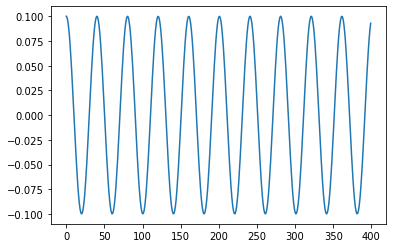
phi_0 = 0.1                              #Angle initial[deg]

phi=phi_0*cos(np.sqrt(g/l)*t)
plt.plot(phi)

x = l * sin(phi)       
y = -l * cos(phi)      

fig, ax = plt.subplots()

line, = ax.plot([], [], 'o-', linewidth=2) 

def animation(i):
    thisx = [0, x[i]]
    thisy = [0, y[i]]

    line.set_data(thisx, thisy)
    return line,

ani = FuncAnimation(fig, animation, frames=np.arange(0, len(t)), interval=25, blit=True)

ax.set_xlim(-l,l)
ax.set_ylim(-l,l)
ax.set_aspect('equal')
ax.grid()
ani.save('pendulum.gif', writer='pillow', fps=15)
plt.show()

vibration

g = 10                                 #Accélération gravitationnelle[m/s^2]
l = 1                                 #Longueur du pendule[m]

def models(t, state):#Équation du mouvement
    dy = np.zeros_like(state)
    dy[0] = state[1]
    dy[1] = -(g/l)*sin(state[0])
    return dy

t_span = [0,20]                         #Temps d'observation[s]
dt = 0.05                               #intervalle[s]
t = np.arange(t_span[0], t_span[1], dt)
phi_0 = 90.0                              #Angle initial[deg]
omega_0 = 0.0                                #Vitesse angulaire initiale[deg/s]

state = np.radians([phi_0, omega_0])           #Etat initial

results = solve_ivp(models, t_span, state, t_eval=t)
phi = results.y[0,:]

plt.plot(phi)

x = l * sin(phi)       
y = -l * cos(phi)      

fig, ax = plt.subplots()

line, = ax.plot([], [], 'o-', linewidth=2) #Dessinez en attribuant des coordonnées à cette ligne l'une après l'autre

def animation(i):
    thisx = [0, x[i]]
    thisy = [0, y[i]]

    line.set_data(thisx, thisy)
    return line,

ani = FuncAnimation(fig, animation, frames=np.arange(0, len(t)), interval=25, blit=True)

ax.set_xlim(-l,l)
ax.set_ylim(-l,l)
ax.set_aspect('equal')
ax.grid()
plt.show()

ani.save('pendulum.gif', writer='pillow', fps=15)

Chapitre 2

Si les coordonnées des points de qualité sont respectivement ($ x_1, y_1 ) et ( x_2, y_2 $), l'énergie cinétique de ce système est

T=\frac{m_1}{2}(\dot{x_1}^2+\dot{y_1}^2)+\frac{m_2}{2}(\dot{x_2}^2+\dot{y_2}^2) L'énergie de la position U=m_1gy_1+m_2gy_2 En outre, les conditions contraignantes sont x_1^2+y_1^2=l_1^2, (x_2-x_1)^2+(y_2-y_1)^2=l_2^2 Est. Il est nécessaire d'utiliser la constante indécise de Lagrange pour résoudre l'équation cinétique du lagrangien. Par conséquent, nous utiliserons également des coordonnées polaires dans ce cas.

x_1=l_1\sin \theta_1 y_1=l_1\cos \theta_1 x_2=l_1\sin \theta_1+l_2\sin \theta_2 y_2=l_1\cos \theta_1+l_2\cos \theta_2

Puisque $ l_1 et \ l_2 $ sont constants, chacun est différencié dans le temps. \dot{x_1}=l_1\dot{\theta_1}\cos \theta_1 \dot{y_1}=-l_1\dot{\theta_1}\sin \theta_1 \dot{x_2}=l_1\dot{\theta_1}\cos \theta_1+l_2\dot{\theta_2}\cos \theta_2 \dot{y_2}=-l_1\dot{\theta_1}\sin \theta_1-l_2\dot{\theta_2}\sin \theta_2 Énergie d'exercice T_1=\frac{m_1}{2}l_1^2\dot{\theta_1}^2(\sin^2\theta_1+\cos^2\\theta_1)=\frac{m_1}{2}l_1^2\dot{\theta_1}^2 T_2=\frac{m_2}{2}[(l_1\dot{\theta_1}\sin\theta_1 +l_2\dot{\theta_2}\sin\theta_2 )^2+(-l_1\dot{\theta_1}\cos\theta_1-l_2\dot{\theta_2}\cos\theta_2 )^2] \ =\frac{m_2}{2}(l_1^2\dot{\theta_1}^2\sin^2\theta_1+2l_1l_2\dot{\theta_1}\dot{\theta_2}\sin\theta_1\sin\theta_2+l_1^2\dot{\theta_2}^2\sin^2\theta_2+l_1^2\dot{\theta_1}^2\cos^2\theta_1+2l_1l_2\dot{\theta_1}\dot{\theta_2}\cos\theta_1\cos\theta_2+l_1^2\dot{\theta_2}\cos^2\theta_2) \ =\frac{m_2}{2} (l_1^2\dot{\theta_1}^2+2l_1l_2\dot{\theta_1}\dot{\theta_2}\cos(\theta_1-\theta_2)+l_1^2\dot{\theta_2}^2) T=T_1+T_2=\frac{m_1+m_2}{2}l_1^2\dot{\theta_1}^2+\frac{m_2}{2}(2l_1l_2\dot{\theta_1}\dot{\theta_2}\cos(\theta_1-\theta_2)+l_1^2\dot{\theta_2}^2) L'énergie de la position U_1=-m_1gl_1\cos\theta_1 U_2=-m_2g(l_1\cos\theta_1+l_2\cos\theta_2) U=U_1+U_2=-(m_1+m_2)gl_1\cos\theta_1-m_2gl_2\cos\theta_2 Par conséquent, Lagrangean L=T-U=\frac{m_1+m_2}{2}l_1^2\dot{\theta_1}^2+\frac{m_2}{2}(2l_1l_2\dot{\theta_1}\dot{\theta_2}\cos(\theta_1-\theta_2)+l_2^2\dot{\theta_2}^2)+(m_1+m_2)gl_1\cos\theta_1+m_2gl_2\cos\theta_2

Pour trouver l'équation du mouvement d'Euler Lagrangian \frac{\partial L}{\partial \theta_1}=-m_2l_1l_2\dot{\theta_1}\dot{\theta_2}\sin(\theta_1-\theta_2)+(m_1+m_2)gl_1\sin\theta_1

\frac{d}{dt}\frac{\partial L}{\partial \dot{\theta_1}}=\frac{d}{dt}[(m_1+m_2)l_1^2\dot{\theta_1}+m_2l_1l_2\dot{\theta_2}\cos(\theta_1-\theta_2)] \ = (m_1+m_2)l_1^2\ddot{\theta_1}+m_2l_1l_2\ddot{\theta_2}\cos(\theta_1-\theta_2)

\frac{\partial L}{\partial \theta_2}=m_2l_1l_2\dot{\theta_1}\dot{\theta_2}\sin(\theta_1-\theta_2)-m_2gl_2\sin\theta_2 \frac{d}{dt}\frac{\partial L}{\partial \dot{\theta_2}}=\frac{d}{dt}[m_2l_1l_2\dot{\theta_1}\cos(\theta_1-\theta_2)+m_2l_2^2\dot{\theta_2})] \ = m_2l_1l_2\ddot{\theta_1}\cos(\theta_1-\theta_2)+m_2l_2^2\ddot{\theta_2}

\therefore m_2l_1l_2\dot{\theta_1}\dot{\theta_2}\sin(\theta_1-\theta_2)-(m_1+m_2)gl_1\sin\theta_1 = (m_1+m_2)l_1^2\ddot{\theta_1}+m_2l_1l_2\ddot{\theta_2}\cos(\theta_1-\theta_2)

m_2l_1l_2\dot{\theta_1}\dot{\theta_2}\sin(\theta_1-\theta_2)-m_2gl_2\sin\theta_2= m_2l_1l_2\ddot{\theta_1}\cos(\theta_1-\theta_2)-m_2l_2^2\ddot{\theta_2}

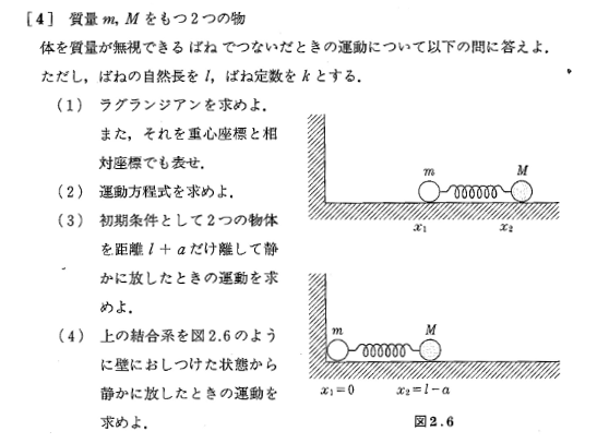
Exercices p.20-21

(1) Puisque la force appliquée à l'objet A est $ (kx) $, l'énergie de position $ U = -kx ^ 2 $, l'énergie cinétique $ T = \ frac {1} {2} m \ dot {x} ^ 2 $ Force appliquée à l'objet B $ kmg $, $ U = Mgx $, énergie cinétique $ T = \ frac {1} {2} M \ dot {x} ^ 2 $

Donc, L=\frac{1}{2}(m+M)\dot{x}^2-\frac{1}{2}kx^2+Mgx Suivant $ \frac{\partial L}{\partial \dot{x}}=(m+M)\dot{x}$ $ \frac{d}{dt}\frac{\partial L}{\partial \dot{x}}=(m+M)\dot{x}$ $ \frac{\partial L}{\partial x}=-kx+Mg$ Plus l'équation de mouvement de Lagrangian ((m+M)\ddot{x}=-kx+Mg or (m+M)\ddot{x_1}=kx_1 (1) Où $ x_1 = -x + Mg / k $

Puisque la solution générale de l'équation (1) est $ A \ sin (\ omega t + \ alpha) $ x_1=A \sin(\omega t + \alpha) (2) \dot{x_1}=\omega A \cos(\omega t + \alpha) (3)

Si $ t = 0 $ $ x = 0 $, donc $ x_1 = -Mg / k $, $ \ dot {x} = 0 $, donc $ \ dot {x_1} = 0 $ x_1(0)=A \sin(\alpha)=-Mg/k \dot{x_1(0)}=\omega A \cos( \alpha)=0

\ cos (\ alpha) = 0 $ pour $ \ omega A \ cos (\ alpha) = 0 \therefore \alpha=90^o

x_1(0)=A\sin(90^O)=A=-\frac{Mg}{k}, \therefore A=-Mg/k

\frac{\partial x_1}{\partial t} = -\omega \frac{Mg}{k} \cos(\omega t + \alpha)

x_1=-\frac{Mg}{k} \sin(\omega t+90^o) \frac{\partial x_1}{\partial t} = -\omega \frac{Mg}{k} \cos(\omega t + \alpha) \frac{\partial \dot{x_1}}{\partial t^2} = -\omega^2 \frac{Mg}{k} \sin(\omega t + \alpha)=x_1\omega^2 \ddot{x_1}=-x_1 \omega^2 Par conséquent, à partir de (1) -\omega^2(m+M)x_1=-kx_1 \omega=\sqrt{\frac{k}{m+M}}

x=\frac{M}{k}g(1-\cos\sqrt{\frac{k}{m+M}}t)

(1)

En coordonnées relatives

La force agissant sur la promesse

F=-kdx=k(l-x_2-x_1)

Énergie potentielle

U=\frac{1}{2}k(l-x_2-x_1)^2

Énergie d'exercice

T=\frac{1}{2}m\dot{x_1}^2+\frac{1}{2}M\dot{x_2}^2

U=\frac{1}{2}k((l-x)^2

Sera. Donc,

L=T-U=\frac{1}{2}m\dot{x_1}^2+\frac{1}{2}M\dot{x_2}^2-\frac{1}{2}k((l-x)^2

Dans les coordonnées du centre de gravité

Avec $ X = \ frac {mx_1 + Mx_2} {m + M} $ comme centre de gravité, $ x = x_2-x_1 $, $ \ dot {X} = \ frac {m \ dot {x_1} + M \ dot { x_2}} {m + M} $

\dot{X}^2=\frac{m^2\dot{x_1}^2+2mM\dot{x_1}\dot{x_2}+M^2\dot{x_2}^2}{(m+M)^2}

Parce que ça devient

T=\frac{1}{2}m\dot{x_1}^2+\frac{1}{2}M\dot{x_2}^2

\ \ =\frac{1}{2}(m+M)\dot{X}^2+\frac{1}{2}\frac{mM}{m+M}\dot{x}^2

Sera. Donc

L=\frac{1}{2}(m+M)\dot{X}^2+\frac{1}{2}\frac{mM}{m+M}\dot{x}^2-\frac{1}{2}((l-x_2-x_1)^2

(2)

L'équation du mouvement de Lagrange

$\frac{d}{dt}\frac{\partial L}{\partial \dot{x_i}} = \frac{\partial L}{\partial x_i} $

Parce qu'il est représenté par

En coordonnées relatives

M\ddot{x_2}=k(l-x)

Dans les coordonnées du centre de gravité

(M+m)\ddot{X}=0

\frac{mM}{m+M}\ddot{x}=k(l-x)

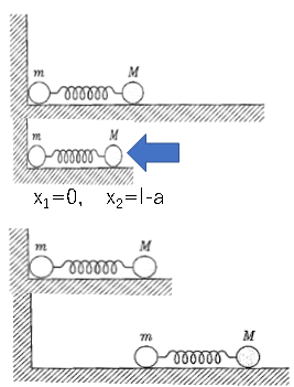
(3) Séparer deux objets par une distance de $ l + a $ signifie $ x_2-x_1-l = a $, donc si vous intégrez $ (M + m) \ ddot {X} = 0 $ une fois

\dot{X}=C

Si vous intégrez à nouveau

X=Ct+D

Par conséquent, il se déplace linéairement avec le passage du temps.

Aussi,

$ \ frac {mM} {m + M} \ ddot {x} = -k ((l-x) $ à $ A sin (wt + \ alpha) $

Si $ x_3 = x-l $, alors $ x_3 (t) = A sin (wt + \ alpha) $

Donc

\dot{x_3}(t)=-w A cos(wt+\alpha)

\ddot{x_3}(t)=-w^2 A sin(wt+\alpha)=-w^2 x_3

\frac{mM}{m+M}\ddot{x_3}=\frac{mM}{m+M}(-w^2 x_3)=-kx_3

Donc,

$w^2=\frac{k(m+M)}{mM} $

par conséquent

$w=\sqrt{\frac{k(m+M)}{mM}} $

x_3=A sin (wt+\alpha)

Quand $ t = 0 $

$ x_3 (0) = A sin (\ alpha) = 1 $ Donc $ A = a $

$ \ dot {x_3} (0) = w A cos (\ alpha) = 0 $ Donc $ \ alpha = 90 ^ o $

Donc

x_3=A sin (wt+90^o)=a cos(wt)=a cos(\sqrt{\frac{k(m+M)}{mM}}t)

\because

x=a cos(\sqrt{\frac{k(m+M)}{mM}}t)+l

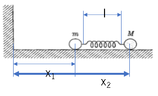
Jusqu'à ce que la promesse s'éloigne du mur

En coordonnées relatives

$T=\frac{1}{2}M\dot{x_2}^2 $

U=\frac{1}{2}l(l-x_2)

Sera. Donc

L=\frac{1}{2}M\dot{x_2}^2-\frac{1}{2}(l-x_2)

L'équation du mouvement de Lagrange

M\ddot{x_2}=-k(x_2-l)

Si $ x_3 = l-x_3 $

M\ddot{x_3}=kx_3

Donc,

x_3(t)=A sin (wt+\alpha)

\dot{x_3}(t)=-wA cos (wt+\alpha)

\ddot{x_3}(t)=-w^2A sin (wt+\alpha)=-w^2 x_3

M \ddot{x_3}=M(-w^2x_3)=-kx_3

\because \ w=\sqrt{\frac{k}{M}}

Lorsque $ t = t_0 $

$ A sin (w t_0 + \ alpha) = a $ puis $ A = a $ Et $ \ alpha = \ pi / 2 $

Donc,

w t_0 +\alpha=\pi \because t_0=\frac{\pi}{2}\sqrt{\frac{M}{k}}

Après $ t_0 $, l'exercice est calculé dans (2). Cependant, remplacez-le par $ t = t-t_0 $.

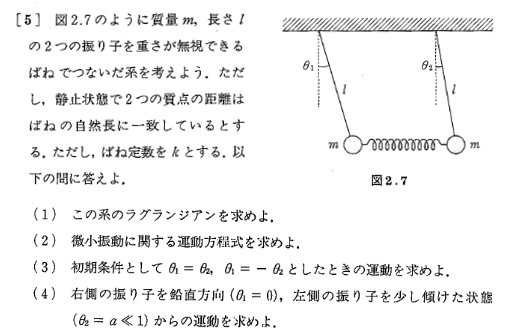
(1)

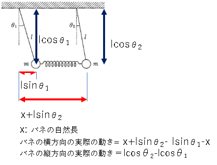
Position des points de qualité le long de l'axe des x: x_1=l \cdot sin \theta_1 x_2=x+l \cdot sin \theta_2

Position des points de qualité le long de l'axe y: y_1=l \cdot cos \theta_1 y_2=l \cdot cos \theta_2

Par conséquent, la différenciation temporelle de premier ordre est \dot{x_1}=-l \cdot cos \theta_1 \dot{\theta_1} \dot{x_2}=-l \cdot cos \theta_2 \dot{\theta_2} \dot{y_1}=l \cdot sin \theta_1 \dot{\theta_1} \dot{y_2}=l \cdot sin \theta_2 \dot{\theta_2} Par conséquent, l'énergie cinétique est $ \frac{1}{2}m(\dot{x_1}^2+\dot{x_2}^2+\dot{y_1}^2+\dot{y_2}^2)=$ $ \frac{1}{2}ml^2(\cdot cos^2 \theta_1 \dot{\theta_1}^2+\cdot cos^2 \theta_2 \dot{\theta_2}^2+ \cdot sin^2 \theta_1 \dot{\theta_1}^2+\cdot sin^2 \theta_2^2 \dot{\theta_2}^2)= \frac{1}{2}ml^2 (\dot{\theta_1}^2+\dot{\theta_2}^2)$

L'énergie potentielle de la source U_1=\frac{1}{2}k(x_2-x_1)^2+(y_2-y_1)^2=\frac{1}{2}kl^2[(sin \theta_2-sin \theta_1)^2+(cos \theta_2-cos \theta_1)^2]

L'énergie de la position U_2=mg(y_1+y_2)=mgl(cos \theta_1+ cos \theta_2)

Par conséquent, Lagrangean

L=\frac{1}{2}ml^2(\dot{\theta_1}^2+\dot{\theta_2}^2)+mgl(cos \theta_1+ cos \theta_2)-\frac{1}{2}kl^2[(sin \theta_2-sin \theta_1)^2+(cos \theta_2-cos \theta_1)^2]

(2) Puisqu'il s'agit d'une vibration minuscule, si $ \ theta_1 <1, \ \ theta_2 <1, \ omega_g ^ 2 = g / l, \ omega_k ^ 2 = k / m $, elle peut être approximée comme $ sin \ theta = \ theta $. De L'énergie potentielle de la source U_1=\frac{1}{2}kl^2(\theta_2-\theta_1)^2 Aussi, \frac{d}{dt}\frac{\partial L}{\partial \dot{\theta_1}}=ml\ddot{\theta_1} \frac{d}{dt}\frac{\partial L}{\partial \dot{\theta_2}}=ml\ddot{\theta_2} \frac{\partial U_1}{\partial \theta_1}=-kl^2(\theta_2-\theta_1) \frac{\partial U_1}{\partial \theta_2}=kl^2(\theta_2-\theta_1) \frac{\partial U_2}{\partial \theta_1}=-mgl sin\theta_1=-mgl\theta_1 \frac{\partial U_2}{\partial \theta_1}=-mgl sin \theta_2=-mgl\theta_2 Donc, \ddot{\theta_1}=\omega_g^2\theta_1-2\omega_k^2(\theta_2-\theta_1) \ddot{\theta_2}=\omega_g^2\theta_2+2\omega_k^2(\theta_2-\theta_1)

(3) Si la valeur initiale est $ \ theta_1 = \ theta_2 $, les deux points de qualité se déplacent dans le même sens, alors ajoutez les formules ci-dessus ensemble. \ddot{\theta_1}+\ddot{\theta_2}=-\omega_g^2(\theta_1+\theta_2) Par conséquent, la fréquence angulaire est $ \ omega = \ omega_g $ Si la valeur initiale est $ \ theta_1 = - \ theta_2 $, les deux points de qualité se déplacent dans des directions opposées, donc la différence entre les équations ci-dessus est \ddot{\theta_1}-\ddot{\theta_2}=-\omega_g^2(\theta_1-\theta_2)-2\omega_k^2(\theta_1-\theta_2) Par conséquent, la fréquence angulaire est $ \ omega = \ sqrt {\ omega_g ^ 2 + 2 \ omega_k ^ 2} $ Sera.

(4) Puisque la valeur initiale est $ \ theta_1 = 0, \ \ theta_2 = a $, la somme des angles du ressort maintient $ a $, donc $ \ theta_1 + \ theta_2 = a $, la différence d'angle est Gardez $ \ theta_1- \ theta_2 = -a $.