[PYTHON] First TensorFlow-Linear Regression as an Introduction
** (Addition: I posted a revised article --http://qiita.com/TomokIshii/items/0a7041ad337f68f71286) **
Last week (November 9, 2015), Deep Learnin's Framework "TensorFlow" was released, but I was convinced that the explanation of the document "MNIST (classification of handwritten numbers) is" Hello World "of machine learning." I can't. As was the case with Coursera's Machine Learning (Stanford), when learning machine learning from the beginning, I personally think of it as Linear Regression at first.
In this article, we will first examine the code for Linear Regression and then create the code for Logistic Regression to get a feel for TensorFlow.
Linear Regression
Regarding "Theano", which is the forerunner of TensorFlow (released first), the Newmu Theano-Tutorials code is published on GitHub in addition to the tutorial of the original document. (https://github.com/Newmu/Theano-Tutorials)
Some short codes are posted so that you can get a better understanding of "Theano" step by step. Next to 0_multiply.py (multiplication), 1_linear_regression.py (linear regression code) is posted, but based on this Theano version, we will create the TensorFlow version code.
First is the Theano version of the code.
#Symbolic variable definition"T"Is theano.Replacing tensor
X = T.scalar()
Y = T.scalar()
def model(X, w):
    return X * w
#Declaration of shared variables
w = theano.shared(np.asarray(0., dtype=theano.config.floatX))
y = model(X, w)
#Graph definition
cost = T.mean(T.sqr(y - Y))
gradient = T.grad(cost=cost, wrt=w)
updates = [[w, w - gradient * 0.01]]
#function
train = theano.function(inputs=[X, Y], outputs=cost, updates=updates, allow_input_downcast=True)
#Learning by loop calculation
for i in range(100):
    for x, y in zip(trX, trY):
        train(x, y)
Next, let's take a closer look at the TensorFlow version.
First, after importing the related modules, prepare the data to be used. (Theano version was test data without intercept b, but here it is included b (= 3.0).)
import numpy as np
import tensorflow as tf

trX = np.linspace(-1, 1, 101)
trY = 2 * trX + 3 + np.random.randn(*trX.shape) * 0.33

def lin_model(X, w, b):
    return X * w + b
lin_model () is a function used as a regression model. (A linear function with slope w and intercept b as parameters.)
Next, prepare the necessary variables.
w = tf.Variable([0.])
b = tf.Variable([0.])

x = tf.placeholder(tf.float32, shape=(101))
y = tf.placeholder(tf.float32, shape=(101))
w and b are ordinary variables. The initial value was set to [0.]. Although x and y are terms unique to TensorFlow (terminology), they are prepared as placeholders. Since it is a placeholder, there is no actual value at the time of declaring this, and the actual value is assigned in the subsequent program processing.
Then we describe the important relationship between variables called Graph.
y_hypo = lin_model(x, w, b)
cost = tf.reduce_mean(tf.square(y_hypo - y))
cost is a cost function that corresponds to the difference between your model and the actual data. "tf.reduce_mean ()" is a function that calculates the mean. (I think "mean ()" is fine, but in TensorFlow it is "reduce_mean ()" for some reason ... It seems that it is in the Reduction function group.)
Then define the Optimizer specification and its method for the calculation of the parameter search.
train_step = tf.train.GradientDescentOptimizer(0.01).minimize(cost)
Here, the gradient descent Optimizer is specified, and the learning rate of 0.01 is given as an argument.
About Optimizer
Now, I'm curious about Optimizer, but TensorFlow currently supports the following. http://www.tensorflow.org/api_docs/python/train.html#optimizers
| Optimizer name | Description |
|---|---|
| GradientDescentOptimizer | Gradient descent optimizer |
| AdagradOptimizer | AdaGrad method optimizer |
| MomentumOptimizer | Momentum optimizer |
| AdamOptimizer | Adam method (This is also famous.) |
| FtrlOptimizer | (I heard it for the first time)"Follow the Regularized Leader"algorithm |
| RMSPropOptimizer | (I heard it for the first time) An algorithm that automates the adjustment of the learning rate |
The parameters that must be set differ depending on the Optimizer, but this time we will use the basic GradientDescentOptimizer. (The required parameter learning rate was set as described above.)
Linear Regression (continued)
Now that we are almost ready, we start a Session that shows the main computational part. However, the variables (Variables) must be initialized before starting the Session. This is unique to "TensorFlow", which was not in "Theano".
# Initializing
init = tf.initialize_all_variables()
"Initializing Variables before the start of Session" seems to be a rule that is often forgotten. For the time being, if you check --The variable of tf.Variable () needs to be initialized **. --The variable of tf.placeholder () is initialized ** not required **. (It will be assigned to the entity later) --The variables (constants) of tf.constant are not initialized **. It is said that. In the list above, variables are initialized using initialize_all_variable ().
The Session part is as follows.
# Train
with tf.Session() as sess:
    sess.run(init)

    for i in range(1001):
        sess.run(train_step, feed_dict={x: trX, y: trY})
        if i % 100 == 0:
            print "%5d:(w,b)=(%10.4f, %10.4f)" % (i, sess.run(w), sess.run(b))
There seem to be several ways to write a program to run Sessoin, but as mentioned above, the session delimiter becomes clear by enclosing it in the "with" statement, and it is automatically opened when you exit "with". Session is closed (), which is convenient.
One is that it is difficult to give Train data in TensorFlow. How to give data (Data Feeding) is the part where the processing changes depending on how to proceed with learning, but as shown in the above list, "feed-dict" will be used, so keep in mind. (I'm still studying this part ...)
With the above, the regression parameters are calculated. (It is shown how it is used for the true values w = 2.0 and b = 3.0.)
    0:(w,b)=(    0.0135,     0.0599)
  100:(w,b)=(    0.9872,     2.6047)
  200:(w,b)=(    1.4793,     2.9421)
  300:(w,b)=(    1.7280,     2.9869)
  400:(w,b)=(    1.8538,     2.9928)
  500:(w,b)=(    1.9173,     2.9936)
  600:(w,b)=(    1.9494,     2.9937)
  700:(w,b)=(    1.9657,     2.9937)
  800:(w,b)=(    1.9739,     2.9937)
  900:(w,b)=(    1.9780,     2.9937)
 1000:(w,b)=(    1.9801,     2.9937)
The above is summarized and the program is posted again. (The program has about 30 lines.)
import numpy as np
import tensorflow as tf

trX = np.linspace(-1, 1, 101)
trY = 2 * trX + 3 + np.random.randn(*trX.shape) * 0.33

def lin_model(X, w, b):
    return X * w + b

w = tf.Variable([0.])
b = tf.Variable([0.])

x = tf.placeholder(tf.float32, shape=(101))
y = tf.placeholder(tf.float32, shape=(101))
y_hypo = lin_model(x, w, b)

cost = tf.reduce_mean(tf.square(y_hypo - y))
train_step = tf.train.GradientDescentOptimizer(0.01).minimize(cost)

# Initializing
init = tf.initialize_all_variables()

# Train
with tf.Session() as sess:
    sess.run(init)

    for i in range(1001):
        sess.run(train_step, feed_dict={x: trX, y: trY})
        if i % 100 == 0:
            print "%5d:(w,b)=(%10.4f, %10.4f)" % (i, sess.run(w), sess.run(b))
About Interactive Session
The above list is a program that executes Session as a batch process (albeit short). Apart from this, TensorFlow supports a function called Interactive Session, which, as the name implies, allows you to move interactively. http://tensorflow.org/get_started/basic_usage.html#interactive-usage
This means that it works well with IPython, that is, it works well with Jupyter Notebook, so I immediately tried it.
(It is like this...)
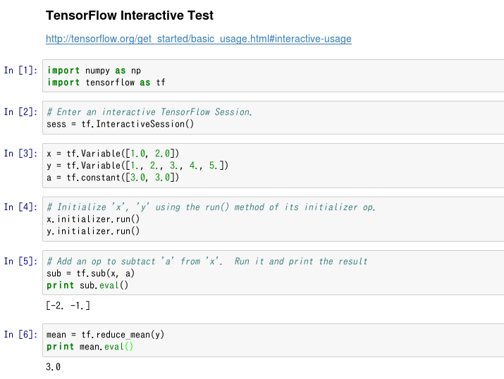
This kind of usage seems to be convenient when trying to study TensorFlow from now on. (On the contrary, this Interactive Session is not suitable for the case of executing a program for a long time.)
Logistic Regression
Based on the above Linear Regression code, we created the Logistic Regression code. Note that this code is for two-class classification, not for multiple classes. (As you know, MNIST uses Softmax regression, which does the problem of multiclass (10 class) classification.)
 def lin_model(X, w, b):
    return X * w + b

w = tf.Variable([0.])
b = tf.Variable([0.])

x = tf.placeholder(tf.float32, shape=(mlen))
y = tf.placeholder(tf.float32, shape=(mlen))

p_1 = lin_model(x, w, b)
x_entropy = tf.nn.sigmoid_cross_entropy_with_logits(p_1, y, name='xentropy')
loss = tf.reduce_mean(x_entropy, name='xentropy_mean')

train_step = tf.train.GradientDescentOptimizer(0.5).minimize(loss)
In Linear Regression, the cost function defined by Mean Square Error (MSE) is replaced with cross entropy in Logistic Regression. "Tf.nn.sigmoid_cross_entropy_with_logits ()" in the second half of the above list is a function that calculates cross entorpy. ("TensorFlow" has many long-named functions ...)
Initialization of variables (Variables) and how to proceed with Session are the same as the previous code.
So far, we have seen the codes for linear regression and logistic regression. At this point, I think we can start working on MLP (Multi Layer Perceptron) code (for example, MNIST) smoothly.
References (web site)
- TensorFlow web site http://www.tensorflow.org/
- Newmu Theano-Tutorials - GitHub https://github.com/Newmu/Theano-Tutorials --Try regression with TensorFlow --Qiita http://qiita.com/syoamakase/items/db883d7ebad7a2220233 --Enjoy Coursera / Machine Learning materials twice --Qiita http://qiita.com/TomokIshii/items/b22a3681cb17836c8f6e
(Note) The TenforFlow document seems to be updated frequently, probably because the version is still shallow. Please forgive me if the link is broken.
Recommended Posts