[PYTHON] [Statistics] First "standard deviation" (to avoid frustration with statistics)
For those who want to learn statistics from now on, I think there is a "standard deviation" that is a very important concept but difficult to understand. I'm familiar with it up to the "average", and I think it feels like "I understand", but the "standard deviation" that suddenly appears.
\sigma = \sqrt{ {1 \over n} \sum_{i=1}^n(x_i - \bar{x})^2}
Wall of. I think there are some people who have been overwhelmed by the fact that "math is impossible" around here.
If you post the image of the graph first, the length of the red line below is the "standard deviation". We will also clarify why this length is the standard deviation.
 (code is here)
In this article, I will explain what the standard deviation is from 1 so that even those who are not good at mathematics can understand it. I will explain it so that even those who understand the formula but do not understand the meaning of "standard deviation" can intuitively understand it, so please have a look.
(* In this article, $ n $ is used as the denominator of the standard deviation. There are cases where $ n-1 $ is used, and it is used properly depending on the case to be analyzed, but here, the one with the simplest notation is $. I will explain using n $.)
</ i> 0. About symbols
If you are unfamiliar with mathematics, you will stumble upon mathematical symbols. What is "$ x_i $"?
\sum_{i=1}^n x_i
This is an explanation for those who are refreshing. If you are OK with mathematical symbols around here, please jump to [Next Section](http://qiita.com/kenmatsu4/items/e6c6acb289c02609e619#1 average first anyway).
First, let's start with $ x_i $.
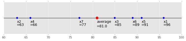
Everyone uses Excel, right? First, suppose you have data for such a test.
| name | Math |
|---|---|
| Tanaka:smile: | 96 |
| Takahashi:flushed: | 63 |
| Suzuki:stuck_out_tongue: | 85 |
| Watanabe:stuck_out_tongue_winking_eye: | 66 |
| Shimizu:laughing: | 91 |
| Kimura:grin: | 89 |
| Yamamoto:smirk: | 77 |
In total
Total score=Tanaka(Math) +Takahashi(Math) +Suzuki(Math) +Watanabe(Math) +Shimizu(Math) +Kimura(Math) +Yamamoto(Math)
\\
 = 96 + 63 + 85 + 66 + 91 + 89 + 77 = 567
Can be calculated.
If the ID is used instead of the name,
| ID | Math |
|---|---|
| 1 | 96 |
| 2 | 63 |
| 3 | 85 |
| 4 | 66 |
| 5 | 91 |
| 6 | 89 |
| 7 | 77 |
Total score=  {\rm ID}:1(Math) + {\rm ID}:2(Math) + {\rm ID}:3(Math) + {\rm ID}:4(Math) + {\rm ID}:5(Math) + {\rm ID}:6(Math) + {\rm ID}:7(Math)
\\
 = 96 + 63 + 85 + 66 + 91 + 89 + 77 = 567
is. Try replacing the score with a variable instead of a number. The score for a person with ID: 1 will be $ x_1 $. The number at the bottom right represents the ID. Then, the formula for the total score is
Total score=  {\rm ID}:1(Math) + {\rm ID}:2(Math) + {\rm ID}:3(Math) + {\rm ID}:4(Math) + {\rm ID}:5(Math) + {\rm ID}:6(Math) + {\rm ID}:7(Math)
\\
 = x_1 + x_2 + x_3 + x_4 + x_5 + x_6 + x_7
\\
 = 96 + 63 + 85 + 66 + 91 + 89 + 77 = 567
Is expressed as. Up to this point, there were 7 data, so I should have steadily arranged the additions as described above, but when there are 1000 data, it's not very good, but I can't write it.
That's where $ \ sum $ comes in handy!
Total points=  {\rm ID}:1(Math) + {\rm ID}:2(Math) + {\rm ID}:3(Math) + {\rm ID}:4(Math) + {\rm ID}:5(Math) + {\rm ID}:6(Math) + {\rm ID}:7(Math)
\\
 = x_1 + x_2 + x_3 + x_4 + x_5 + x_6 + x_7
\\
 = \sum_{i=1}^7 x_i
\\
 = 96 + 63 + 85 + 66 + 91 + 89 + 77 = 567
It is expressed as. In other words

So
\sum_{i=1}^7 x_i = x_1 + x_2 + x_3 + x_4 + x_5 + x_6 + x_7
Will be. This way even when there are 1000 data
\sum_{i=1}^{1000} x_i = x_1 + x_2 + \cdots + x_{1000}
It is used because it is convenient because it can be expressed as.
In the first place, if the number is decided in advance, it is not impossible to write 1000 pieces in a row, but the number of data is not known at this time, and even when temporarily placed as $ n $ pieces for the time being ,
\sum_{i=1}^{n} x_i
You can write even if you haven't decided! Convenient!
By the way, if you know how to express it in code, you may know that it is the following process. The $ \ sum $ symbol is a process of turning and adding with a for statement.
sum.py
x = [96, 63, 85, 66, 91, 89, 77]
total = 0
for i in range(len(x)):
    total += x[i]
print total
</ i> 1. Anyway, first of all, average
Let's think about the "average" again. There are different types of averages, such as "arithmetic mean", "geometric mean", and "harmonic mean", but the so-called familiar "average" is the "arithmetic mean".
It's all the data added together and divided by that number. In statistics, this "average" is expressed as $ \ bar {x} $, and the definition is as follows. The number of data is $ n $. In the example of the math test in the previous section, the data is for 7 students, so $ n = 7 $.
\bar{x} = {1 \over n} \sum_{i=1}^{n} x_i
(If you don't understand the meaning of the symbol, please check [previous section](http://qiita.com/kenmatsu4/items/e6c6acb289c02609e619#0 symbol))
The graph is as follows. This is intuitive: blush:
 (code is here)
</ i> 2. What is "deviation"?
Next, I will explain the concept of "deviation". As you can see, "standard ** deviation **" is a little closer to the core.
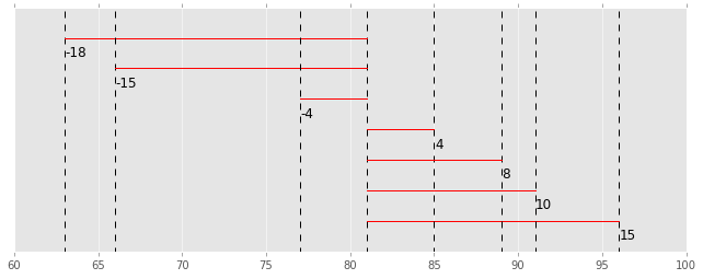
Deviation is the difference between each data and the mean, as shown below.
| ID | Score | deviation |
|---|---|---|
| 1 | 96 | 96-81= 15 |
| 2 | 63 | 63-81= -18 |
| 3 | 85 | 85-81= 4 |
| 4 | 66 | 66-81= -15 |
| 5 | 91 | 91-81= 10 |
| 6 | 89 | 89-81= 8 |
| 7 | 77 | 77-81= -4 |
This is also represented by a graph. The red line is the deviation of each data.
<!-The standard value of this deviation is the "standard deviation". ->
 (code is here)
</ i> 3. Average deviation
Before moving on to standard deviation, I would like to introduce "mean deviation", which is easy to understand intuitively.
This is the average of the "deviations" explained in the previous section. In other words
| ID | deviation |
|---|---|
| 1 | 15 |
| 2 | -18 |
| 3 | 4 |
| 4 | -15 |
| 5 | 10 |
| 6 | 8 |
| 7 | -4 |
I think about the average of, but there is only one problem, and if you add all of them, it will be 0.
What i want to do
Since it is the average length of the red line of, the minus is omitted.
In other words, the minus part of this length ...
 Invert.

| ID | Absolute value of deviation |
|---|---|
| 1 | 15 |
| 2 | 18 |
| 3 | 4 |
| 4 | 15 |
| 5 | 10 |
| 6 | 8 |
| 7 | 4 |
The average value of this "absolute value of deviation" is ** 10.57 **, which is called the "mean deviation". this is,
- Average distance from average
- An indicator of how far you are from the average
It is considered. In this example, the average score is 81 points, but the average score is 10.57 points. It is no exaggeration to say that this concept is almost the idea of standard deviation. Only the computational approach is slightly different. So, when you say "standard deviation", I would like you to have the image of "the average of how far you are from the average".
Express this using mathematical formulas.
First, the absolute value symbol,
When written in a graph, it is expressed like this, and the slope is inverted so that the value becomes positive in the area where $ x $ is negative.
 (code is here)
Expressed in a mathematical formula, it looks like this.

It can be interpreted that the deviation is created by subtracting the average from the value of the data, the minus is removed by taking the absolute value, and the average is taken.
It looks like this in Python code.
mean_deviation.py
x = [96, 63, 85, 66, 91, 89, 77]
ave = np.average(x)
total = 0
for i in range(len(x)):
    total += abs(x[i] - ave)
print total/len(x)
</ i> 4. Standard deviation
Finally, the main character of this article, "standard deviation". In "mean deviation", the absolute value was used to change minus to plus, but in "standard deviation", it was squared and minus was taken. In other words, the idea is exactly the same, only the negative removal method is different.
As shown below, there is a similarity in that the origin is symmetrical with the origin as the folding point, and the negative value is changed to positive.

(code is here)
(The blue line is the absolute value function
In the previous section, as shown in the figure below, the difference from the average value was expressed by the length of the line.

This time, the image of evaluating the difference by the square is to evaluate the degree of deviation from the average value with the area of the square as shown here.

Let's add up these areas and take the average.

Expressing this as a mathematical formula,

The sum of the squares of the deviations from the average and the average is called the "variance". At this point, the "standard deviation" is just one step away.
The formula shown at the beginning of this article is reprinted as follows.
\sigma = \sqrt{ {1 \over n} \sum_{i=1}^n(x_i - \bar{x})^2}
The difference from "dispersion" is whether or not to calculate the route. "Dispersion" is also an indicator of how much data is scattered, but the unit has changed because we are thinking about the area. So you can get the area back to length by taking the root $ \ sqrt {\ } $.
By defining that root $ \ sqrt {\ } $ is the value when squared, $ \ sqrt {9} = \ sqrt {3 ^ 2} = 3 $ or $ \ sqrt {25} = \ sqrt Represents the relationship {5 ^ 2} = 5 $. It's the reverse calculation of $ 3 ^ 2 = 9 $. Since $ 25 $ can be thought of as the area of a square of $ 5 \ times5 $,

If you write it in a mathematical formula, it will look like this. Calculate root $ \ sqrt {\ } $ for the entire variance. You can think of it as an "operation to extract the length of the side" with respect to the average value of the above area.
That is, the standard deviation is
standard deviation= \sqrt{Distributed}
It becomes.
It looks like this in Python code.
standard_deviation.py
x = [96, 63, 85, 66, 91, 89, 77]
ave = np.average(x)
total = 0
for i in range(len(x)):
    total += (x[i] - ave)**2
print np.sqrt(total/len(x))
Also, the reason why I changed it to "square" instead of "absolute value" is a little difficult, but since the processing of the absolute value used for mean deviation is mathematically difficult to handle, I adopted a square that is easy to handle. One point is that it was done. After that, as a concept of distance, it is rather natural to take a route by squared Three squares theorem. I think that is also one of the reasons.
Summary
- Mathematical handling becomes convenient
- Because the concept of distance can be defined as squared and routed in the first place
I think. (A little more detailed explanation will be given in another article: grin :)
</ i> 5. Example 1: Understanding with a graph
As I posted at the beginning, I will write an example in a graph. The average of this data is represented by a red circle, the deviation from the average of each data is calculated, and the standard deviation is further calculated from it and expressed by the length of the red bar.
The image is that the average distance from the average value of all data is the length of this red bar. Since the data is made to be generated over a wider range, the length of the standard deviation bar will also increase.
(code is here)
</ i> 6. Example 2: Deviation value
It is a familiar deviation value for university entrance exams, but this deviation value is also made based on the "standard deviation".
Calculate the mean and standard deviation from the data of all the people who took the test. And
- The average score is 50 deviations
- Deviation value 60 for those who scored one standard deviation higher than the average
- Deviation value 40 for those who scored one standard deviation lower than the average
Calculate as follows. In other words
Deviation value= { (Score-average) \over standard deviation} \times 10 + 50
It is a value calculated as follows. If the score is higher than the average by the length of the red bar in the graph in the previous section, the deviation value is 60!
</ i> Finally
What did you think? I tried to explain it as carefully as possible, but when I reorganized it, I realized again that it is a concept that is composed of quite a variety of elements intertwined. However, if I can understand each element properly, I think that I can have an overall intuition.
I hope that understanding of this standard deviation will make people think "statistics is interesting!" And increase the number of people who are interested in data analysis!
(* If there is a part that says "I don't know", please leave it in the comment section!)
I also wrote an article (slide) entitled "Basics of Statistics", so please refer to this as a related article if you like. http://qiita.com/kenmatsu4/items/5a59a7375140f29b31c2
Recommended Posts