[PYTHON] Finding the beginning of Abenomics from NT magnification 1
Pairs Trade using NT magnification
Pairs Trade is a well-known trading method that uses two stocks that behave similarly. When there is a difference between the two movements, it is a method of trying to make a profit by taking a position that fills the difference, and it is also done by hedge funds.
The method is explained in detail in the recently read "Time-series data analysis that can be used immediately in the field", and theoretically, it seems that the relationship between the two cointegrations is a prerequisite for establishing pair trading. At first, I wanted to do a Back Test to see if I could make a profit. In Japan, the NT magnification is taken up as a material for pair trading, but as some of you may know, the ratio of the two indexes, Nikkei225 and Topix, is called the NT magnification (= Nikkei225 / Topix). The question arises as to whether the combination of indexes is "theoretical", but I decided to look at it as a popular method.
In the process of investigating, I saw a big change in Trend, so I thought about it under the title of "Investigating the beginning of Abenomics".
Historical Chart and Scatter Plot
First is the observation of time series data.

Both Topix and Nikkei225 are stock indexes calculated from the stock prices of the first section of the Tokyo Stock Exchange, so the movements are very similar. The y-axis scale is different in the Chart (Nikkei225-left, Topix-right), but the lines almost overlap from 2005 to 2009. You can also see the Trend where the Nikkei 225 has moved up from the Topix line since around 2010.
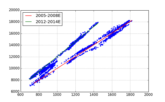
Next, let's look at Scatter Plot.

In this Chart, we can see that the plot is along the neighborhood of two straight lines. Considering this together with the first plot and Historical Chart, it can be inferred that the straight line with the smaller slope was the trend of NT at first, but over time, it changed to the trend with the larger slope. Based on this idea, we then performed a regression analysis. By the way, the Historical Chart of the NT magnification itself is as follows.

Regression analysis with Stats Models
This time, we performed linear regression analysis, but the Python module used ** StatsModels **. From the time series data of (Topix, Nikkei225), data was extracted by setting two time intervals, and regression was performed for each. The time intervals are 2005 / B ~ 2008 / E and 2012 / B ~ 2014 / E. The former is the time before the "Lehman shock" occurs, and the latter is the era of so-called "Abenomics".
import statsmodels.api as sm
# ... pre-process ...

# Regression Analysis
index_s1 = pd.date_range(start='2005/1/1', end='2008/12/31', freq='B')
x1 = pd.DataFrame(index=index_s1); y1 = pd.DataFrame(index=index_s1)

x1['topix'] = mypair['topix']   # 2005 .. 2008/E
y1['n225'] = mypair['n225']

x1 = sm.add_constant(x1)
model1 = sm.OLS(y1[1:], x1[1:])
mytrend1 = model1.fit()
print mytrend1.summary()

index_s2 = pd.date_range(start='2012/1/1', end='2014/12/31', freq='B')
x2 = pd.DataFrame(index=index_s2); y2 = pd.DataFrame(index=index_s2)

x2['topix'] = mypair['topix']   # 2012 .. 2014/E
y2['n225'] = mypair['n225']

x2 = sm.add_constant(x2)
model2 = sm.OLS(y2[1:], x2[1:])
mytrend2 = model2.fit()
print mytrend2.summary()

# Plot fitted line
plt.figure(figsize=(8,5))
plt.plot(mypair['topix'], mypair['n225'], '.')
plt.plot(x1.iloc[1:,1], mytrend1.fittedvalues, 'r-', lw=1.5, label='2005-2008E')
plt.plot(x2.iloc[1:,1], mytrend2.fittedvalues, 'g-', lw=1.5, label='2012-2014E')
plt.grid(True)
plt.legend(loc=0)
After setting each data in the DataFrame object called mypair [['topix','n225']] in pandas, the above list was executed.
I was able to fit the two straight lines neatly. Although it is an evaluation of regression analysis, it shows a number that exceeds expectations. (Both regression calculations have good results, but one result is shown.)
>>> print mytrend1.summary()
        OLS Regression Results (Early period, 2005-2008E)
==============================================================================
Dep. Variable:                   n225   R-squared:                       0.981
Model:                            OLS   Adj. R-squared:                  0.981
Method:                 Least Squares   F-statistic:                 5.454e+04
Date:                Sun, 21 Jun 2015   Prob (F-statistic):               0.00
Time:                        17:11:26   Log-Likelihood:                -7586.3
No. Observations:                1042   AIC:                         1.518e+04
Df Residuals:                    1040   BIC:                         1.519e+04
Df Model:                           1
==============================================================================
                 coef    std err          t      P>|t|      [95.0% Conf. Int.]
------------------------------------------------------------------------------
const        -45.0709     62.890     -0.717      0.474      -168.477    78.335
topix         10.0678      0.043    233.545      0.000         9.983    10.152
==============================================================================
Omnibus:                       71.316   Durbin-Watson:                   0.018
Prob(Omnibus):                  0.000   Jarque-Bera (JB):               30.237
Skew:                          -0.189   Prob(JB):                     2.72e-07
Kurtosis:                       2.256   Cond. No.                     8.42e+03
==============================================================================
Warnings:
[1] The condition number is large, 8.42e+03. This might indicate that there are
strong multicollinearity or other numerical problems.
The coefficient of determination R-squired is 0.981, F-stat 5.454e + 04 p-value 0.00 (!). As mentioned above, the conditional numer is too large from the program, isn't it strange? of Warning has occurred. (This time, I haven't pursued this Warning deeply ... Please give me any advice.)
The equations of the two Trend Lines obtained from this regression analysis (coef) are as follows. Period-1(2005-2008) : n225 = topix x 10.06 - ** 45.07 ** Period-2(2012-2014) : n225 = topix x 12.81 - 773.24
It can be said that the index of NT magnification has changed from ** 10.06 ** to ** 12.81 **. However, one question is why this big change is not visible in NT's Historical Chart.

Since the intercept changed from Period-1 to Period-2, I also searched for'ntr2'(green line) that eliminated the effect, but it was said that NT jumped in a staircase pattern (from 10.06 to 12.81). It doesn't seem to be the case.
The conclusion from the analysis so far is that ** "Abenomics began between 2009 and 2012 (early)" **. It's not a neat result, but it's natural (from this result) to think that this economic trend had already begun, at least in December 2012, when Prime Minister Abe took office as Prime Minister for the second term.
(Since the conclusion is not clear, I did the classification using scikit-learn next. See the article "2".)
References
-"Time-series data analysis that can be used immediately in the field" (Daisuke Yokouchi (Author), Yoshimitsu Aoki (Author), Gijutsu-Hyoronsha) http://gihyo.jp/book/2014/978-4-7741-6301-7
- "Python for Finance": (O'reilly Media) http://shop.oreilly.com/product/0636920032441.do --pandas documentation http://pandas.pydata.org/pandas-docs/stable/index.html --StatsModels documentation http://statsmodels.sourceforge.net/stable/
Recommended Posts