[PYTHON] Observe TCP congestion control with ns-3
1.First of all
Most traffic on the Internet is said to be controlled by ** TCP (Transmission Control Protocol) **. One of the features of TCP is that each transmitting node adjusts the amount of data transmitted at one time based on the ** congestion control algorithm **. In this article, ns-3 simulates the behavior of each algorithm, and NumPy + [matplotlib] Visualize with (http://matplotlib.org/).
To compare TCP congestion control algorithms, ns-3 has [tcp-variants-comparison.cc](https://www.nsnam.org/docs/release/3.26/doxygen/tcp-variants- A sample scenario called comparison_8cc.html) is prepared. However, if this scenario script is used as it is, there is a problem that some variables of interest in this article cannot be monitored (in ns-3, they are called ** trace **). Therefore, in this article, we will introduce how to add arbitrary trace information to the scenario script.

The source code for this article is all on Github.
[^ Congestion]: It is a word of the image of congestion in the network.
2. Environment construction
2.1 ns-3 (Network Simulator 3) ns-3 is an open source discrete event network simulator. Developed for use in research and educational purposes. This article assumes the environment and directory structure built in the following article.
Network simulation starting with ns-3.26
2.2 python In this article, NumPy is used for data processing, and matplotlib is used for graph drawing. We have confirmed the operation in the following environment.
- Python 2.7.11
- NumPy 1.10.4
- matplotlib 1.5.1
3. Congestion control in TCP
3.1 Overview
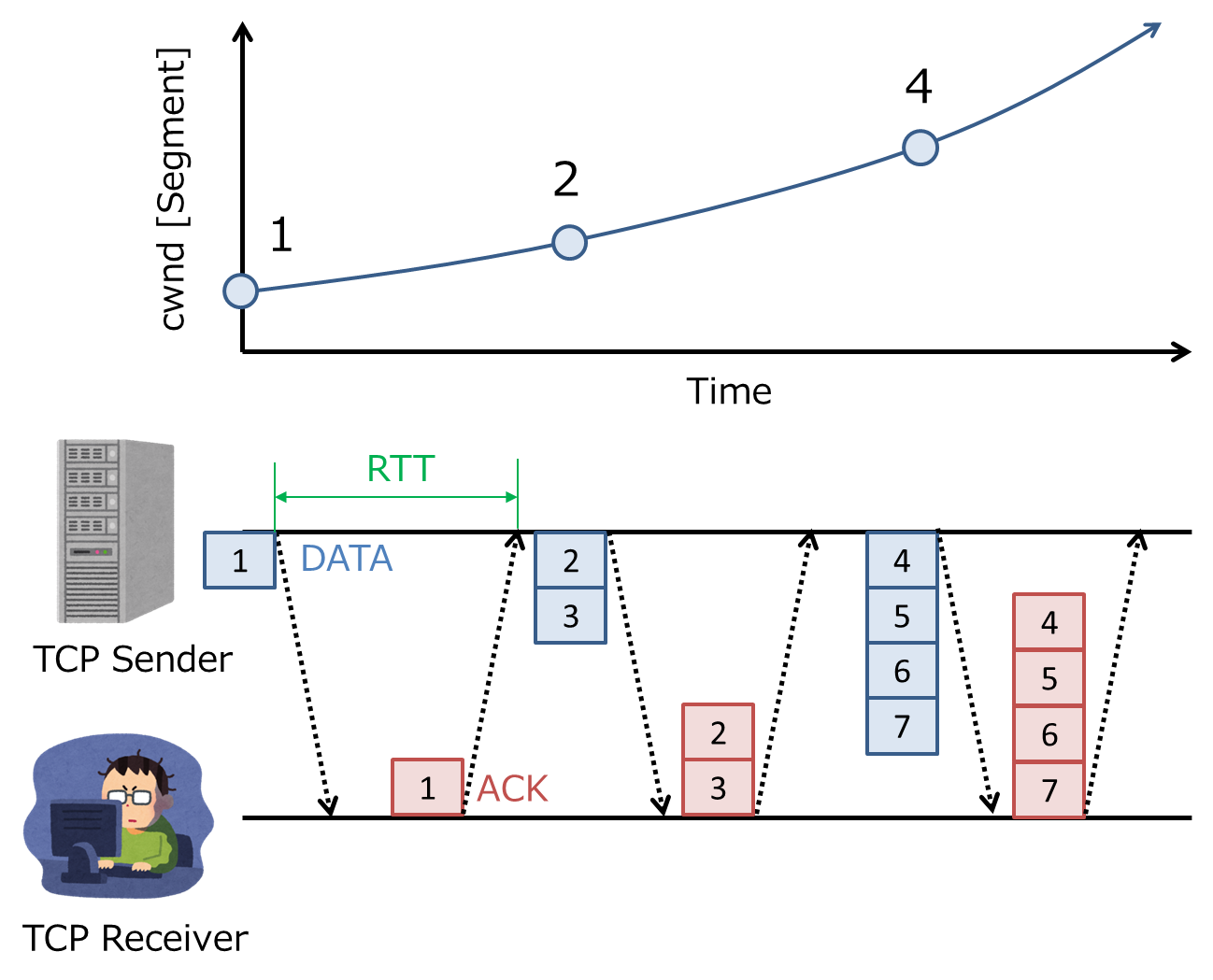
The figure below is an image of TCP congestion control assumed in this article. The TCP transmitting node (TCP Sender) has the amount of data according to the acknowledgment (Acknowledgement, ACK) [^ delayed ACK] [^ ACK number] from the receiving node (TCP Receiver) and the signal round trip time (Round Trip Time, RTT). Adjust (DATA).
[^ delayed ACK]: To simplify the explanation, this article does not consider delayed ACK (delayed acknowledgement). Delayed ACK is a method that improves network utilization efficiency by transmitting multiple ACKs at once.
[^ ACKnumber]: Acknowledgement number is strictly the received Sequence number + Segment size. In this article, in order to make the explanation intuitive, we use an image diagram that ACKs the segment number of DATA as it is.
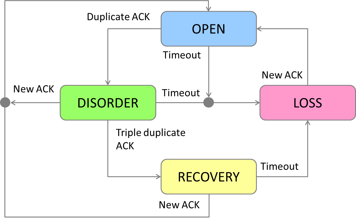
Strictly speaking, the adjustment of the amount of data can be expressed by the formula $ swnd = min (awnd, cwnd) $. Here, $ swnd $ is the upper limit of the number of DATA that TCP Sender can send without ACK, $ cwnd $ is the window size (Congestion window) that TCP Sender adjusts autonomously, and $ and $ is TCP. This is the window size (Advertised window) announced by Receiver. The unit of the above formula is called a segment, and the size of one segment is determined by the negotiation between TCP Sender and Receiver. Since $ awnd $ is often set to a very large value, for the sake of simplicity, we will focus only on $ cwnd $ in this article. The larger $ cwnd $, the more data can be sent at once. TCP Sender predicts how busy the network is with the Receiver from ACK and RTT, and autonomously adjusts the size of $ cwnd $. The adjustment strategy for $ cwnd $ is called ** congestion control ** in this article. Congestion control is determined by two factors: ** congestion state [^ state transition diagram] ** (Congestion state) and ** algorithm ** (Congestion control algorithm). Congestion status indicates network congestion status such as * OPEN *, * DISORDER *, * RECOVER *, * LOSS *. The algorithm shows how to update $ cwnd $ in each congestion state.
[^ State transition diagram]: It is different from the so-called TCP state transition diagram (Finite state machine). The state transition diagram covers the process from connection establishment to disconnection, while the congestion state targets the congestion state during connection establishment (ESTABLISHED).
3.2 Congestion state
In this article, the implementation of ns-3 (~ / ns-3.26 / source / ns-3.26 / src / internet / model / tcp-socket-base.cc Based on docs / release / 3.26 / doxygen / tcp-socket-base_8cc.html)), the following four types of congestion are assumed.
-
- OPEN *: This is the so-called normal state. Depending on the algorithm, there are two types of phases, Slow start (SS) and Congestion avoidance (CA). When $ cwnd $ is smaller than the threshold (Slow start threshold, $ ssth $), it corresponds to the Slow start phase, and when it is larger, it corresponds to the Congestion avoidance phase.
-
- DISORDER *: A state in which a duplicate ACK (Duplicate ACK) has been received. There is a possibility of packet loss or disorder of reception order.
-
- RECOVERY *: A state in which a triple duplicate ACK has been received. We are confident of packet loss and start resending.
-
- LOSS *: RTT becomes larger than the retransmission time out (RTO), that is, the ACK timeout is detected. There may be serious congestion.
3.3 Congestion control algorithm
In this article, the following congestion control algorithms are assumed based on the [Implementation] of ns-3 (https://www.nsnam.org/docs/models/html/tcp.html). TypeId is like the name of the algorithm in ns-3. The source code is stored in ~ / ns-3.26 / source / ns-3.26 / src / internet / model respectively.
| algorithm | TypeId |
Source code |
|---|---|---|
| NewReno | TcpNewReno |
tcp-congestion-ops.cc |
| HighSpeed | TcpHighSpeed |
tcp-highspeed.cc |
| Hybla | TcpHybla |
tcp-hybla.cc |
| Westwood | TcpWestwood |
tcp-westwood.cc |
| Westwood+ | TcpWestwoodPlus |
tcp-westwood.cc |
| Vegas | TcpVegas |
tcp-vegas.cc |
| Scalable | TcpScalable |
tcp-scalable.cc |
| Veno | TcpVeno |
tcp-veno.cc |
| Bic | TcpBic |
tcp-bic.cc |
| YeAH | TcpYeah |
tcp-yeah.cc |
| Illinois | TcpIllinois |
tcp-illinois.cc |
| H-TCP | TcpHtcp |
tcp-htcp.cc |
For example, one of the most major congestion control algorithms, New Reno (Reno), updates $ cwnd $ in each congestion state as follows: I will.
| Renewal opportunity | Renewal formula |
|---|---|
| OPENWhen an ACK is received in the (SS) state | $ cwnd \gets cwnd + 1$ |
| OPENWhen an ACK is received in the (CA) state | $ \displaystyle cwnd \gets cwnd + \frac{1}{cwnd}$ |
| RECOVERYWhen transitioning to the state | |
| RECOVERYWhen a duplicate ACK is received in the state | $ \displaystyle cwnd \gets cwnd + 1$ |
| RECOVERYIn the state, receive a new ACK andOPENWhen transitioning to the state | $ cwnd \gets ssth$ |
| LOSSWhen transitioning to the state | $ cwnd \gets smss$, |
Here, $ \ mathit {inflight} $ represents the total amount of DATA for which ACK has not been returned, and $ smss $ represents the minimum segment size. Also, for simplicity, Partial ACK and Full ACK are not considered. For details on the operation of NewReno, refer to RFC6582.
NewReno efficiently transmits DATA by increasing $ cwnd $ at high speed in the Slow start phase where the possibility of congestion is low, while the Congestion avoidance phase where the possibility of congestion is high. In, we have adopted a strategy of avoiding sudden congestion by gradually increasing $ cwnd $.
Please note that the update formula triggered by ACK reception is ** an update formula for ACK for one segment ** (I was addicted to it here). For example, when $ cwnd = 4 $, TCP Sender receives ACK [^ delayedACK] for 4 segments of DATA, so the above update is performed ** 4 times **.
There are three types of TCP implementation in ns-3, but in this article, ns-3 native ( Only the algorithms implemented in src / internet / model) are targeted. In other words, the major CUBIC on Linux and the major CTCP On Windows. uk / ~ lewis / CTCP.pdf) is out of scope. I would like to introduce these separately.
- ns-3 native (
src / internet /) - NSC(Network Simulation Cradle)
- DCE(Direct Code Execution)
[^ ack]: Delayed ACK.
4. Creating a scenario script
In this chapter, we will explain the sample scenario tcp-variants-comparison.cc, its problems, and the modified version my-tcp-variants-comparison.cc.
4.1 Based sample scenario
ns-3 is [tcp-variants-comparison.cc](https://www.nsnam.org/docs/release/3.26/doxygen/tcp-variants-comparison_8cc] for comparison of TCP congestion control algorithms. .html)
We have prepared a sample scenario called (located at ~ / ns-3.26 / source / ns-3.26 / examples / tcp /). This scenario script can trace the time change of the following variables and output it to a file.
- Cwnd: The above $ cwnd $. However, the unit is bytes.
- SsThresh: $ ssth $. However, the unit is bytes.
- Rtt: The RTT. The unit is [s].
- Rto: The above RTO. The unit is [s].
- NextTx: The Sequence number that TCP Sender will send next.
- NextRx: The Sequence number that the TCP Receiver will receive next.
- InFlight: The above $ \ mathit {inflight} $. However, the unit is bytes. Due to the principle of TCP, it is always less than $ cwnd $.
In the following, I will explain the source code, focusing on ** Trace **, which is the theme of this article.
Variables for tracing
Lines 58 to 70 define the variables used for tracing. bool first * indicates whether or not to output the initial value of the trace target, and Ptr <OutputStreamWrapper> * Stream indicates the stream for outputting the trace target to a file, respectively. ʻUint32_t * Value` Represents variables that are temporarily used when dealing with the initial values to be traced.
tcp-variants-comparison.cc (lines 58 to 70)
bool firstCwnd = true;
bool firstSshThr = true;
bool firstRtt = true;
bool firstRto = true;
Ptr<OutputStreamWrapper> cWndStream;
Ptr<OutputStreamWrapper> ssThreshStream;
Ptr<OutputStreamWrapper> rttStream;
Ptr<OutputStreamWrapper> rtoStream;
Ptr<OutputStreamWrapper> nextTxStream;
Ptr<OutputStreamWrapper> nextRxStream;
Ptr<OutputStreamWrapper> inFlightStream;
uint32_t cWndValue;
uint32_t ssThreshValue;
Setting the callback function for tracing
Lines 73 to 145 define the trace callback function * Tracer (), and lines 147 to 202 define the function Trace * () that associates the callback function with the trace target. I will do it. Here, we will explain using BytesInFlight, which is one of the trace targets, as an example.
tcp-variants-comparison.cc (lines 73 to 202)
static void
InFlightTracer (uint32_t old, uint32_t inFlight)
{
  *inFlightStream->GetStream () << Simulator::Now ().GetSeconds () << " " << inFlight << std::endl;
}

//=====Abbreviation=====

static void
TraceInFlight (std::string &in_flight_file_name)
{
  AsciiTraceHelper ascii;
  inFlightStream = ascii.CreateFileStream (in_flight_file_name.c_str ());
  Config::ConnectWithoutContext ("/NodeList/1/$ns3::TcpL4Protocol/SocketList/0/BytesInFlight", MakeCallback (&InFlightTracer));
}
In ns-3, all variables ʻAddTraceSource () in the source file (ns-3.26 / source / ns-3.26 / src / * / model /) are set as trace targets in the scenario script. can. For example, the above BytesInFlight is [~ / ns-3.26 / source / ns-3.26 / src / internet / model / tcp-socket-base.cc](https://www.nsnam.org/docs) /release/3.26/doxygen/tcp-socket-base_8cc.html) ʻAddTraceSource (). Every time the variable to be traced is updated, ns-3 calls the callback function associated with that variable. Therefore, to set the trace target, it is necessary to ** define the callback function ** and ** link the trace target and the callback function **.
As a callback function, a function like ʻInFlightTracer () above is often used. ʻInFlightTracer () is a function that outputs the current time (Simulator :: Now (). GetSeconds ()) and the updated value (ʻinFlight) each time. When associating the trace target with the callback function, you can use the syntax Config :: ConnectWithoutContext (variable, MakeCallback (& func))as described inTraceInFlight ()above. Here,variableneeds to describe the path of the Object to be traced./ NodeList / 1 / $ ns3 :: TcpL4Protocol / SocketList / 0 / BytesInFlight means the variableBytesInFlightofSocketList 0 socket, which hangs from NodeList`1 node.
For details on the tracing method for ns-3, refer to section 1.10 of the Official Manual.
Network configuration
Set the network configuration with main () from the 204th line onward. Details are given to the Official Manual, and only the points are described here.
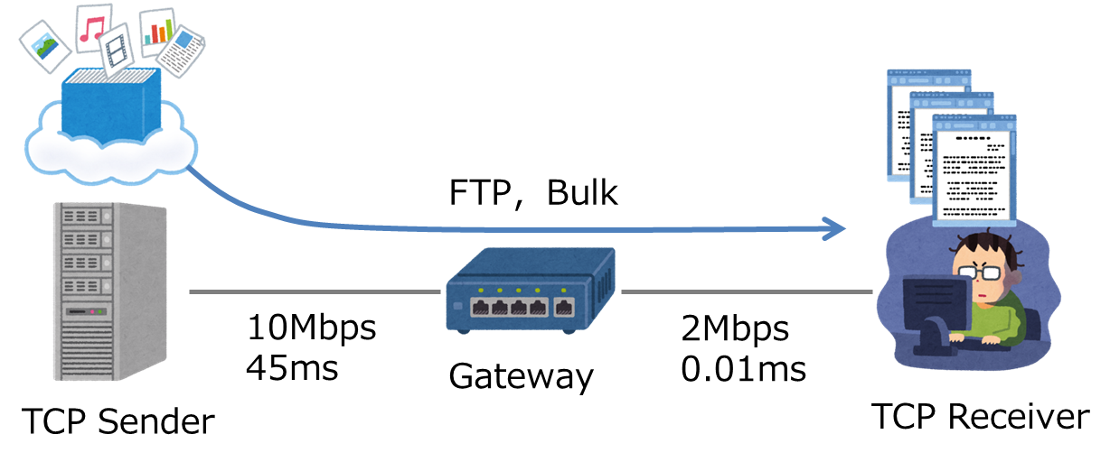
The figure above is an image of this scenario. Imagine a simple configuration with one TCP Sender and one Receiver. Use BulkSendHelper, which simulates a large amount of FTP-like data transmission. The IP packet size is 400 bytes. The simulation time is 100 seconds by default.
Command line arguments
Set command line arguments on lines 224 to 243. As introduced in the previous article (http://qiita.com/haltaro/items/b474d924f63692c155c8), you can set command line arguments by CommandLine.AddValue ().
tcp-variants-comparison.cc (lines 224 to 243)
CommandLine cmd;
  cmd.AddValue ("transport_prot", "Transport protocol to use: TcpNewReno, "
                "TcpHybla, TcpHighSpeed, TcpHtcp, TcpVegas, TcpScalable, TcpVeno, "
                "TcpBic, TcpYeah, TcpIllinois, TcpWestwood, TcpWestwoodPlus ", transport_prot);
  cmd.AddValue ("error_p", "Packet error rate", error_p);
  cmd.AddValue ("bandwidth", "Bottleneck bandwidth", bandwidth);
  cmd.AddValue ("delay", "Bottleneck delay", delay);
  cmd.AddValue ("access_bandwidth", "Access link bandwidth", access_bandwidth);
  cmd.AddValue ("access_delay", "Access link delay", access_delay);
  cmd.AddValue ("tracing", "Flag to enable/disable tracing", tracing);
  cmd.AddValue ("prefix_name", "Prefix of output trace file", prefix_file_name);
  cmd.AddValue ("data", "Number of Megabytes of data to transmit", data_mbytes);
  cmd.AddValue ("mtu", "Size of IP packets to send in bytes", mtu_bytes);
  cmd.AddValue ("num_flows", "Number of flows", num_flows);
  cmd.AddValue ("duration", "Time to allow flows to run in seconds", duration);
  cmd.AddValue ("run", "Run index (for setting repeatable seeds)", run);
  cmd.AddValue ("flow_monitor", "Enable flow monitor", flow_monitor);
  cmd.AddValue ("pcap_tracing", "Enable or disable PCAP tracing", pcap);
  cmd.AddValue ("queue_disc_type", "Queue disc type for gateway (e.g. ns3::CoDelQueueDisc)", queue_disc_type);
  cmd.Parse (argc, argv);
In this article, we will use the following command line arguments in particular.
transport_prot: Congestion control algorithm can be specified. In this article, we will use a shell script to specify all 12 types in order.tracing: You can specify the presence or absence of tracing. Since it isFalseby default, specifyTrue.duration: You can specify the simulation time. The default of 100 seconds is too long, so we will set it to 20 seconds in this article.prefix_name: You can specify the prefix of the output file name. With the default settings, a large number of files will be spit out directly under~ / ns-3.26 / source / ns-3.26 /, so modify it so that it spits out under thedatadirectory.
Scheduling trace settings
From the 460th line to the 476th line, the trace setting function (callback function and the function that associates the trace target) such as the above TraceInFlight () is scheduled.
tcp-variants-comparison.cc (lines 460 to 476)
  if (tracing)
    {
      std::ofstream ascii;
      Ptr<OutputStreamWrapper> ascii_wrap;
      ascii.open ((prefix_file_name + "-ascii").c_str ());
      ascii_wrap = new OutputStreamWrapper ((prefix_file_name + "-ascii").c_str (),
                                            std::ios::out);
      stack.EnableAsciiIpv4All (ascii_wrap);

      Simulator::Schedule (Seconds (0.00001), &TraceCwnd,
                           prefix_file_name + "-cwnd.data");
      Simulator::Schedule (Seconds (0.00001), &TraceSsThresh,
                           prefix_file_name + "-ssth.data");
      Simulator::Schedule (Seconds (0.00001), &TraceRtt,
                           prefix_file_name + "-rtt.data");
      Simulator::Schedule (Seconds (0.00001), &TraceRto,
                           prefix_file_name + "-rto.data");
      Simulator::Schedule (Seconds (0.00001), &TraceNextTx,
                           prefix_file_name + "-next-tx.data");
      Simulator::Schedule (Seconds (0.00001), &TraceInFlight,
                           prefix_file_name + "-inflight.data");
      Simulator::Schedule (Seconds (0.1), &TraceNextRx,
                           prefix_file_name + "-next-rx.data");
    }
In ns-3, you can schedule to execute func (args, ...) at time with the syntax Simulator :: Schedule (time, & func, args, ...).
However, I'm not sure why you shouldn't Trace * () in the local sentence. I think there is probably a problem with the timing of object creation ...
4.2 Issues for tcp-variants-comparison.cc
tcp-variants-comparison.cc is a very well-made scenario script that you can play with just by tweaking the command line arguments. But I can't trace the ACK or congestion conditions that we are interested in!
Fortunately, the variable HighestRxAck for the latest ACK and the variable CongState for the congestion state are tcp-socket-base.cc respectively. release / 3.26 / doxygen / tcp-socket-base_8cc.html) ʻAddTraceSource ()`. Therefore, you can add them to the trace target with only a few changes to the scenario script. In the following, we will introduce the method.
4.3 New scenario script my-tcp-variants-comparison.cc
First, copy the original tcp-variants-comparison.cc to ~ / ns-3.26 / source / ns-3.26 / scratch and rename it to my-tcp-variants-comparison.cc To do.
$ cd ~/ns-3.26/source/ns-3.26
$ cp examples/tcp/tcp-variants-comparison.cc scratch/my-tcp-variants-comparison.cc
In order to add the ACK and congestion status to the trace target, add trace variables, set trace callback functions, and schedule trace settings.
Add trace variables
Add the stream ʻackStreamfor ACK tracing and the streamcongStateStream` for congestion state tracing.
cpp:my-tcp-variants-comparison.cc(tcp-variants-comparison.Equivalent to lines 58 to 70 of cc)
bool firstCwnd = true;
bool firstSshThr = true;
bool firstRtt = true;
bool firstRto = true;
Ptr<OutputStreamWrapper> cWndStream;
Ptr<OutputStreamWrapper> ssThreshStream;
Ptr<OutputStreamWrapper> rttStream;
Ptr<OutputStreamWrapper> rtoStream;
Ptr<OutputStreamWrapper> nextTxStream;
Ptr<OutputStreamWrapper> nextRxStream;
Ptr<OutputStreamWrapper> inFlightStream;
Ptr<OutputStreamWrapper> ackStream; // NEW!
Ptr<OutputStreamWrapper> congStateStream; // NEW!
uint32_t cWndValue;
uint32_t ssThreshValue;
Setting the callback function for tracing
Add the callback function ʻAckTrace ()for ACK tracing and the callback functionCongStateTracer ()for congestion state tracing. The congestion state is the enumeration typeTcpSocketState :: TcpCongState_t defined in tcp-socket-base.h. Also, add the functions TraceAck ()andTraceCongState ()` that associate the above callback function with the variable to be traced, respectively.
cpp:my-tcp-variants-comparison.cc(tcp-variants-comparison.Equivalent to lines 73 to 202 of cc)
static void
AckTracer (SequenceNumber32 old, SequenceNumber32 newAck)
{
  *ackStream->GetStream () << Simulator::Now ().GetSeconds () << " " << newAck << std::endl;
}

static void
CongStateTracer (TcpSocketState::TcpCongState_t old, TcpSocketState::TcpCongState_t newState)
{
  *congStateStream->GetStream () << Simulator::Now ().GetSeconds () << " " << newState << std::endl;
}

//=====Abbreviation=====

static void
TraceAck (std::string &ack_file_name)
{
  AsciiTraceHelper ascii;
  ackStream = ascii.CreateFileStream (ack_file_name.c_str ());
  Config::ConnectWithoutContext ("/NodeList/1/$ns3::TcpL4Protocol/SocketList/0/HighestRxAck", MakeCallback (&AckTracer));
}

static void
TraceCongState (std::string &cong_state_file_name)
{
  AsciiTraceHelper ascii;
  congStateStream = ascii.CreateFileStream (cong_state_file_name.c_str ());
	Config::ConnectWithoutContext ("/NodeList/1/$ns3::TcpL4Protocol/SocketList/0/CongState", MakeCallback (&CongStateTracer));
}
Scheduling trace settings
Finally, schedule the above TraceAck () and TraceCongState ().
cpp:my-tcp-variants-comparison.cc(tcp-variants-comparison.cc Equivalent to lines 460 to 476)
  if (tracing)
    {

// =====Abbreviation=====

      Simulator::Schedule (Seconds (0.00001), &TraceAck, prefix_file_name + "-ack.data"); // NEW!
      Simulator::Schedule (Seconds (0.00001), &TraceCongState, prefix_file_name + "-cong-state.data"); // NEW!
    }
4.4 Compiling my-tcp-variants-comparison.cc
You can compile my-tcp-variants-comparison.cc by doing ./waf in the ~ / ns-3.26 / source / ns-3.26 directory.
$ ./waf
Waf: Entering directory '~/ns-3.26/source/ns-3.26/source/ns-3.26/build'
[ 985/2524] Compiling scratch/my-tcp-variants-comparison.cc
[2501/2524] Linking build/scratch/my-tcp-variants-comparison
Waf: Leaving directory '~/ns-3.26/source/ns-3.26/source/ns-3.26/build'
Build commands will be stored in build/compile_commands.json
'build' finished successfully (3.240s)

Modules built:
antenna                   aodv                      applications
bridge                    brite (no Python)         buildings
click                     config-store              core
csma                      csma-layout               dsdv
dsr                       energy                    fd-net-device
flow-monitor              internet                  internet-apps
lr-wpan                   lte                       mesh
mobility                  mpi                       netanim (no Python)
network                   nix-vector-routing        olsr
point-to-point            point-to-point-layout     propagation
sixlowpan                 spectrum                  stats
tap-bridge                test (no Python)          topology-read
traffic-control           uan                       virtual-net-device
wave                      wifi                      wimax
xgpon (no Python)

Modules not built (see ns-3 tutorial for explanation):
openflow                  visualizer
5. Experiment
5.1 Executing a scenario script
First, create the data storage directory data.
$ mkdir ~/ns-3.26/source/ns-3.26/data
Execute the following shell script to experiment with all 12 types of algorithms. As introduced in the previous article (http://qiita.com/haltaro/items/b474d924f63692c155c8), you can pass the value value to the command line argument ʻarg with --arg = value. I will. transport_prot is the congestion control algorithm, prefix_nameis the prefix of the output file name,tracing is the presence or absence of tracing, and duration` is the simulation time [s].
compare-tcp-algorithms.sh
#!/bin/bash

ALGORITHMS=(TcpNewReno TcpHighSpeed TcpHybla TcpWestwood TcpWestwoodPlus \
 TcpVegas TcpScalable TcpVeno TcpBic TcpYeah TcpIllinois TcpHtcp)

for algo in ${ALGORITHMS[@]}; do
  echo "----- Simulating $algo -----"
  ./waf --run "my-tcp-variants-comparison --transport_prot=$algo --prefix_name='data/$algo' --tracing=True --duration=20"
done
5.2 Observe congestion control for all algorithms
For now, let's plot $ cwnd $ and $ ssth $ of all algorithms and the change of congestion state with the following plot_cwnd_all_algorithms ().
plottcpalgo.py
# -*- coding: utf-8 -*-
#!/usr/bin/env python


import numpy as np
import matplotlib.pyplot as plt

#This is a function for data shaping.
def get_data(algo, variable='cwnd', duration=20.):
    file_name = 'data/Tcp' + algo + '-' + variable + '.data'
    data = np.empty((0, 2)) #Initialization

    #Get the data from the file.
    for line in open(file_name, 'r'):
        data = np.append(
            data, np.array([map(float, line[:-1].split())]),
            axis=0)
    data = data.T

    #Extract only the data below the duration, at the end[duration, data[1,-1]]To
    #add. It is a process to plot beautifully until the duration time.
    data = data[:, data[0] < duration]
    if len(data[0])==0:
        data = np.append(
            data, np.array([[duration, 0]]).T,
            axis=1)
    else:
        data = np.append(
            data, np.array([[duration, data[1, -1]]]).T,
            axis=1)

    return data


def plot_cwnd_all_algorithms(duration=20.):
    algos = ['NewReno', 'HighSpeed', 'Hybla', 'Westwood', 'WestwoodPlus',
             'Vegas', 'Scalable', 'Veno', 'Bic', 'Yeah', 'Illinois', 'Htcp']
    segment = 340 #In this experimental configuration, the segment length is 340 bytes.

    plt.figure(figsize=(15, 10))
    for i, algo in enumerate(algos):
        plt.subplot(3, 4, i + 1)

        #Acquisition of cwnd, ssth, and congestion status data
        cwnd_data = get_data(algo, 'cwnd', duration)
        ssth_data = get_data(algo, 'ssth', duration)
        state_data = get_data(algo, 'cong-state', duration)

        #Colors are different according to the congestion state.
        #OPEN (blue), DISORDER (green), RECOVERY (yellow), LOSS (red)
        plt.fill_between(cwnd_data[0], cwnd_data[1] / segment,
                         facecolor='lightblue') #The initial state is OPEN (blue)
        for n in range(len(state_data[0])-1):
            fill_range = cwnd_data[0] >= state_data[0, n]
            if state_data[1, n]==1: # 1: DISORDER
                plt.fill_between(
                    cwnd_data[0, fill_range], cwnd_data[1, fill_range] / segment,
                    facecolor='lightgreen')
            elif state_data[1, n]==3: # 3: RECOVERY
                plt.fill_between(
                    cwnd_data[0, fill_range], cwnd_data[1, fill_range] / segment,
                    facecolor='khaki')
            elif state_data[1, n]==4: # 4: LOSS
                plt.fill_between(
                    cwnd_data[0, fill_range], cwnd_data[1, fill_range] / segment,
                    facecolor='lightcoral')
            else: # OPEN
                plt.fill_between(
                    cwnd_data[0, fill_range], cwnd_data[1, fill_range] / segment,
                    facecolor='lightblue')

        #Plot of cwnd (solid line) and ssth (dotted line).
        plt.plot(cwnd_data[0], cwnd_data[1] / segment, drawstyle='steps-post')
        plt.plot(ssth_data[0], ssth_data[1] / segment, drawstyle='steps-post',
                 color='b', linestyle='dotted')
        plt.ylim(0, 1200) #Since the initial value of ssth is messed up, set the upper limit with ylim
        plt.title(algo)

    #Save and view diagrams
    plt.savefig('data/TcpAll' + str(duration).zfill(3) + '-cwnd.png')
    plt.show()
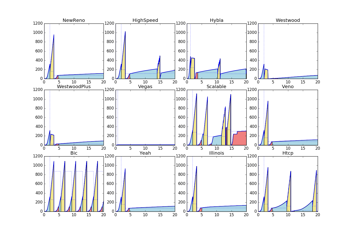
The horizontal axis is time [s] and the vertical axis is $ cwnd $ and $ ssth $ [segment]. $ cwnd $ is a solid line and $ ssth $ is a dotted line. The colors are colored according to the congestion state. $ OPEN $ is blue, $ DISORDER $ is green, $ RECOVERY $ is yellow, and $ LOSS $ is red. The individuality of each algorithm came out more strongly than originally expected.
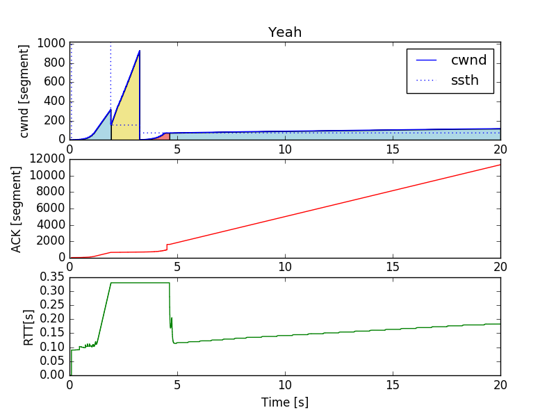
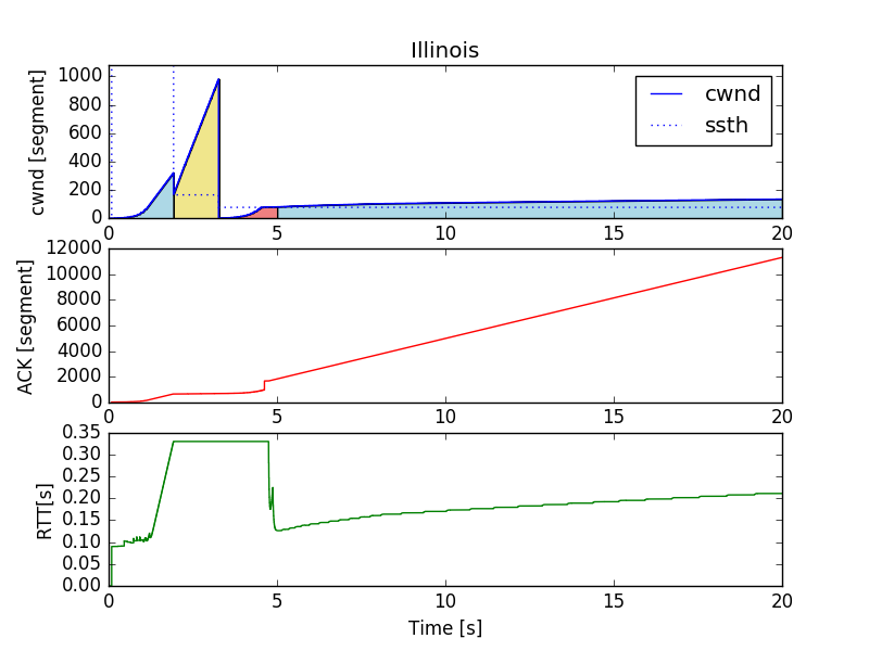
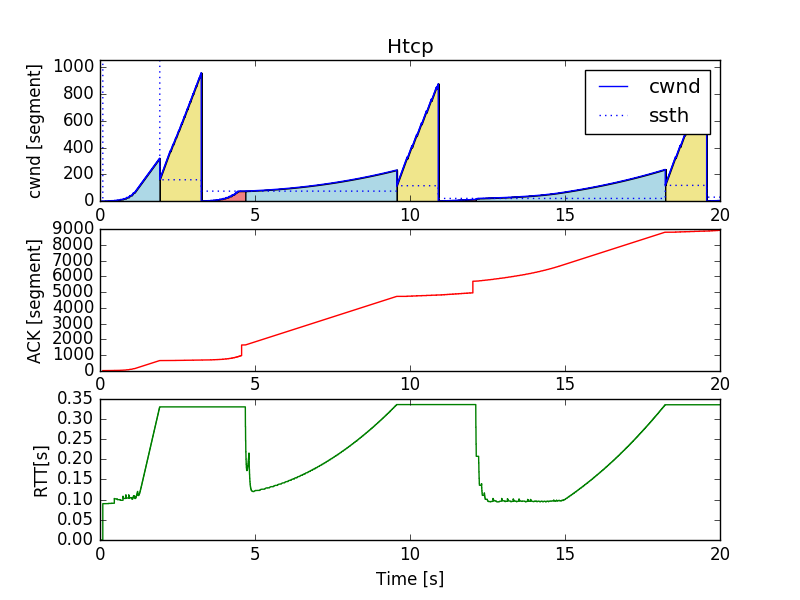
5.3 Observe the relationship between cwnd, ACK, and RTT of each algorithm
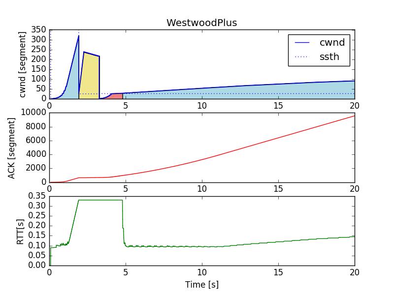
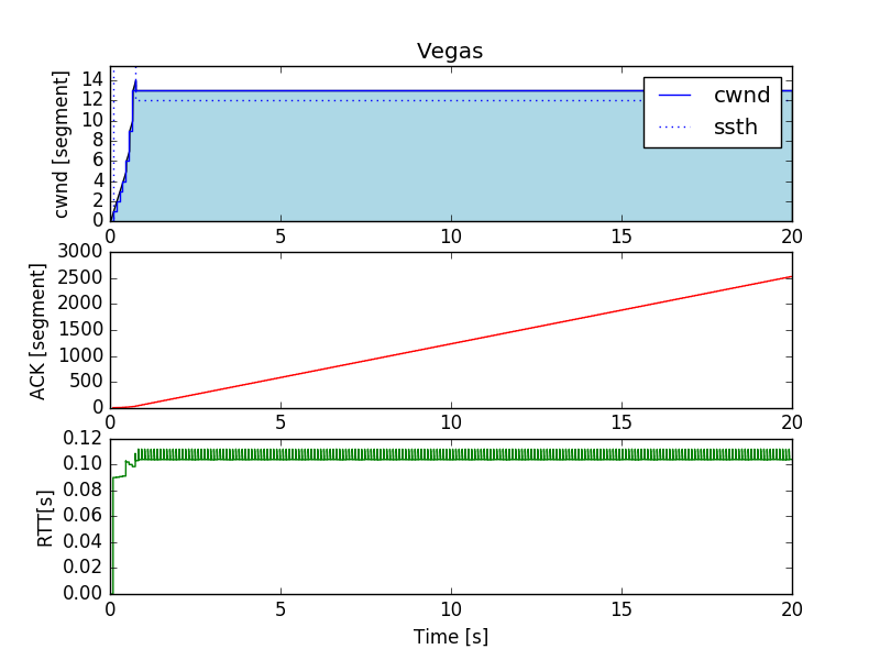
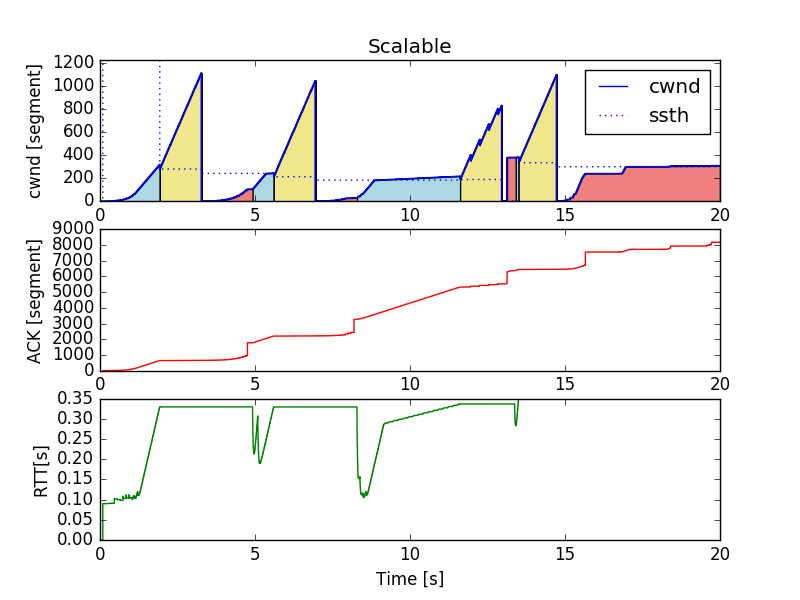
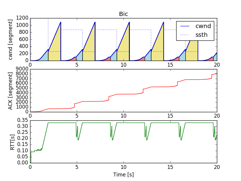
Next, plot $ cwnd $, ACK, and RTT of each algorithm with the following plot_cwnd_ack_rtt_each_algorithm ().
plot_cwnd_ack_rtt_each_algorithm()
def plot_cwnd_ack_rtt_each_algorithm(duration=20.):
    algos = ['NewReno', 'HighSpeed', 'Hybla', 'Westwood', 'WestwoodPlus',
             'Vegas', 'Scalable', 'Veno', 'Bic', 'Yeah', 'Illinois', 'Htcp']
    segment = 340 #In this experimental configuration, the segment length is 340 bytes.
    plt.figure()

    for algo in algos:
        plt.subplot(311) #Plot of cwnd, ssth and congestion state

        #Acquisition of cwnd, ssth, and congestion status data
        cwnd_data = get_data(algo, 'cwnd', duration)
        ssth_data = get_data(algo, 'ssth', duration)
        state_data = get_data(algo, 'cong-state', duration)


        #Colors are different according to the congestion state.
        #OPEN (blue), DISORDER (green), RECOVERY (yellow), LOSS (red)
        plt.fill_between(cwnd_data[0], cwnd_data[1] / segment,
                         facecolor='lightblue') #The initial state is OPEN (blue)
        for n in range(len(state_data[0])-1):
            fill_range = cwnd_data[0] >= state_data[0, n]
            if state_data[1, n]==1: # 1: DISORDER
                plt.fill_between(
                    cwnd_data[0, fill_range], cwnd_data[1, fill_range] / segment,
                    facecolor='lightgreen')
            elif state_data[1, n]==3: # 3: RECOVERY
                plt.fill_between(
                    cwnd_data[0, fill_range], cwnd_data[1, fill_range] / segment,
                    facecolor='khaki')
            elif state_data[1, n]==4: # 4: LOSS
                plt.fill_between(
                    cwnd_data[0, fill_range], cwnd_data[1, fill_range] / segment,
                    facecolor='lightcoral')
            else: # OPEN
                plt.fill_between(
                    cwnd_data[0, fill_range], cwnd_data[1, fill_range] / segment,
                    facecolor='lightblue')

        #Plot of cwnd (solid line) and ssth (dotted line).
        plt.plot(cwnd_data[0], cwnd_data[1] / segment, drawstyle='steps-post',
                 color='b', label='cwnd')
        plt.plot(ssth_data[0], ssth_data[1] / segment, drawstyle='steps-post',
                 color='b', linestyle='dotted', label='ssth')
        ymax = max(cwnd_data[1] / segment)*1.1
        plt.ylim(0, ymax) #Since the initial value of ssth is messed up, set the upper limit with ylim
        plt.ylabel('cwnd [segment]')
        plt.legend()
        plt.title(algo)

        plt.subplot(312) #ACK plot
        ack_data = get_data(algo, 'ack', duration)
        plt.plot(ack_data[0], ack_data[1] / segment, drawstyle='steps-post',
                 color='r')
        plt.ylabel('ACK [segment]')

        plt.subplot(313) #RTT plot
        rtt_data = get_data(algo, 'rtt', duration)
        plt.plot(rtt_data[0], rtt_data[1], drawstyle='steps-post', color='g')
        plt.ylabel('RTT[s]')
        plt.xlabel('Time [s]')

        #Save the image.
        plt.savefig('data/Tcp' + algo + 'Sub-' + str(int(duration)).zfill(3) +
                    '-cwnd-ack-rtt.png')
        plt.clf()
    plt.show()
In the following, we will analyze the results using NewReno as an example. Also, for your reference, the results of other algorithms are also included.
NewReno
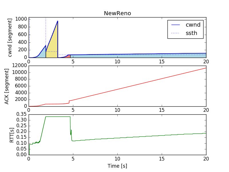
Near 1.93 [s], three duplicate ACKs are received and the state transitions to the $ RECOVERY $ state. To estimate the throughput at this time:
\frac{cwnd}{RTT} \simeq
\frac{321\rm{[segment]} \cdot 340 \rm{[byte/segment] \cdot 8 \rm{[bit/byte]}}}{0.33[s]} \simeq 2.3 \rm{[Mbps]}
Here, the bandwidth of the bottleneck link was 2.0 Mbps (see Section 4.1), so it is not unnatural when congestion occurs [^ analysis]. After transitioning to $ RECOVERY $, you can see that the ACK and RTT updates have stopped. You can also see that the updates to $ cwnd $ and $ ssth $ are consistent with Section 3.3. Around 3.26 [s], it times out without receiving a new ACK and transitions to the $ LOSS $ state. You can see that the updates of $ cwnd $ and $ ssth $ are consistent with Section 3.3. Around 4.69 [s], a new ACK is finally received and the state is transitioning to the $ OPEN $ state.
[^ Analysis]: Maybe. I think more detailed analysis such as queue analysis is needed, but I'm exhausted ...
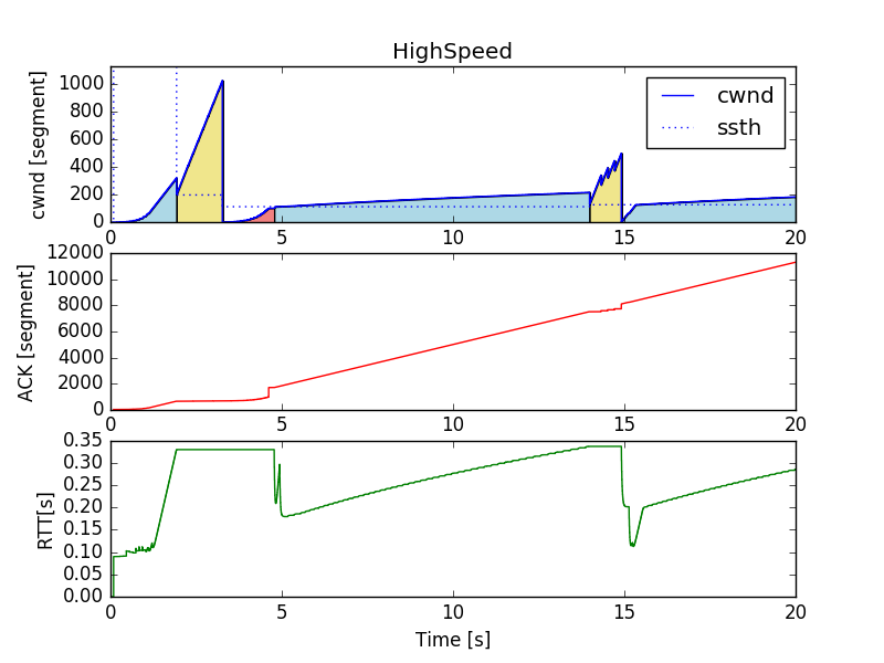
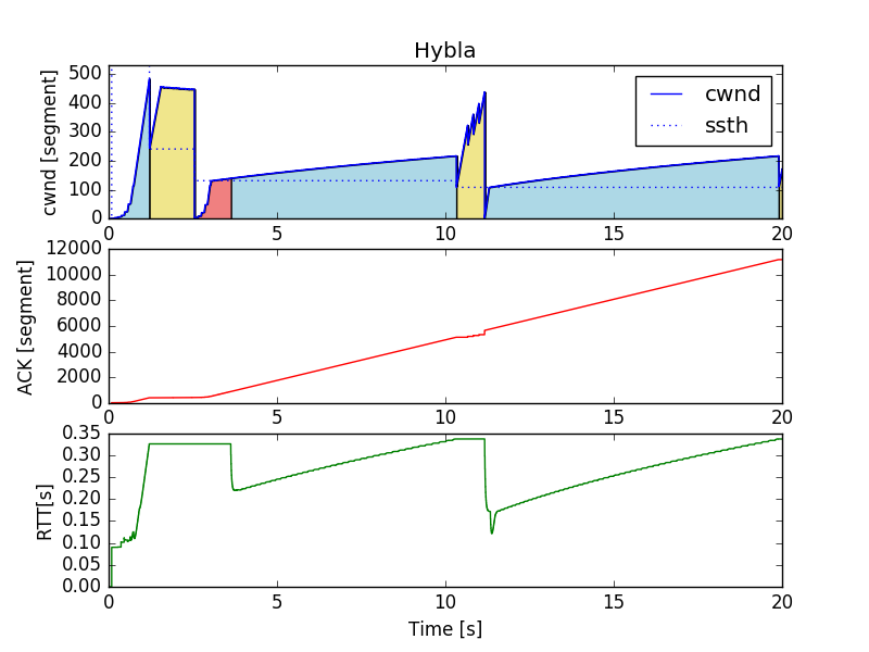
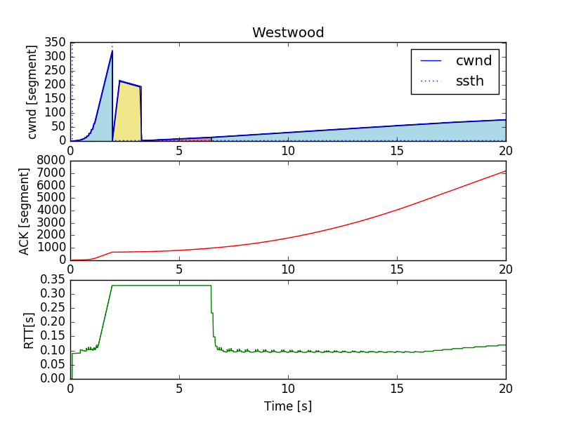
Other algorithms
For your reference, the results of other algorithms are also posted.

6. Conclusion
In this article, I used ns-3 to simulate TCP congestion control and visualized it with python. As a beginner, I was able to get a feel for TCP. We also reaffirmed the excellence of the ns-3 sample scenario. From now on, CUBIC and CTCP I would like to challenge the implementation of major algorithms such as) and the latest algorithms such as Remy. Alternatively, I think it would be good to observe the competition between different algorithms. Thank you for reading to the end!
reference
In creating this article, I referred to the following. Thank you very much!