[PYTHON] RC circuit simulation
I want to calculate the noise level from the voice recorded by the sound level meter
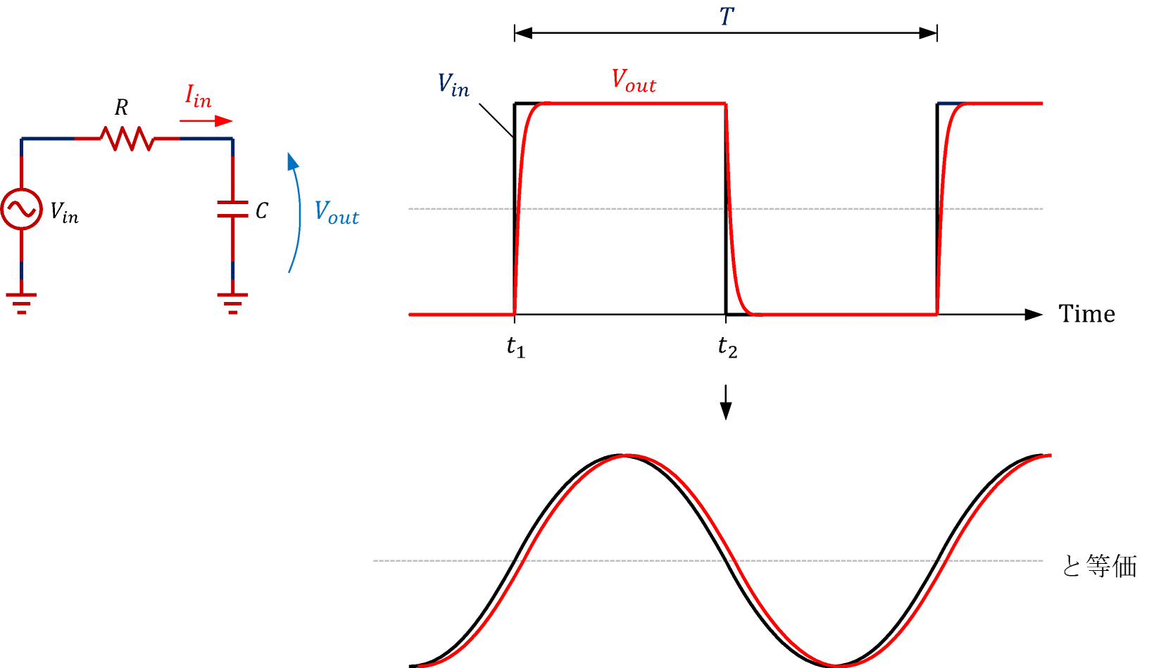
As for the time weighting characteristic of the sound level meter, Fast seems to have a time constant of 125 ms. I did a lot of research to do this in Python, so make a note.
In the sound level meter I'm using, the one in this image I borrowed It seems that the sound pressure squared to $ V_ {in} $ is input and $ V_ {out} $ is output. I didn't do any circuits at all, so I groped around.

I decided to compare it with the output of the following site to confirm whether it was simulated properly. (Amateur doesn't know what is right. By the way, if you think it's a circuit diagram or a picture, you'll be surprised to be able to operate it!) Transient analysis / AC analysis of primary RC circuit
After researching various things, it seems that you can do it with scipy.signal, control.matlab. (At first, both were confused and panicked ...)
Here is the frequency characteristic of the RC circuit you want to simulate.
\begin{align}
\text{Frequency characteristic:}\quad \frac{V_{out}(s)}{V_{in}(s)}&=\frac{1}{1+sCR}\\
\end{align}
Methods to reproduce this are scipy.signal.lsim and control.matlab.lsim //python-control.readthedocs.io/en/0.8.3/generated/control.matlab.lsim.html).
You can create a linear time-invariant system and input any signal to get the output. For scipy, I referred to this site. For example, if you specify $ lti ([a_1, a_2, a_3], [b_1, b_2, b_3]) $ The frequency response is $ \ frac {a_1 s ^ 2 + a_2 s + a_3} {b_1 s ^ 2 + b_2 s + b_3} $ It seems that the number of hours will increase if you arrange the required number. For RC circuits, $ lti ([1], [R * C, 1]) $ is fine.
This is what I was able to do.
RC_circuit_signal.py
from matplotlib import pyplot as plt
import scipy.signal as sg
import numpy as np

R    = 1000        # 1k Ohm(s/F)
C    = 0.000_000_1 # 0.1 F
# 1 / (R * C * s + 1)
num  = [1]
den  = [R * C, 1]
t    = np.linspace(0, 0.01, 1000)
freq = 250
v_in = 0.5 + 0.5 * np.sign(np.sin(2 * np.pi * freq * (t - 0.001)))

system = sg.lti(num, den)
t_out, v_out, x = sg.lsim(system, v_in, t)

plt.style.use('grayscale')
plt.plot(t,     v_in,  label="$V_{in}$")
plt.plot(t_out, v_out, label="$V_{out}$")
plt.xlabel('Time[s]')
plt.ylabel('Amplitude')
plt.legend()
plt.grid()
plt.show()

control.matlab creates a system with control.tf. It looks similar to the previous one, but it looks like this. I don't like the order of the return values of lsim. .. ..
RC_circuit_control_matlab.ipynb
from matplotlib import pyplot as plt
import control.matlab as ctrl
import numpy as np

R    = 1000        # 1k Ohm(s/F)
C    = 0.000_000_1 # 0.1 F
# 1 / (R * C * s + 1)
num  = [1]
den  = [R * C, 1]
t    = np.linspace(0, 0.01, 1000)
freq = 250
v_in = 0.5 + 0.5 * np.sign(np.sin(2 * np.pi * freq * (t - 0.001)))

system = ctrl.tf(num, den)
print(system)
v_out, t_out, x = ctrl.lsim(system, v_in, t)

plt.style.use('grayscale')
plt.plot(t,     v_in,  label="$V_{in}$")
plt.plot(t_out, v_out, label="$V_{out}$")
plt.xlabel('Time[s]')
plt.ylabel('Amplitude')
plt.legend()
plt.grid()
plt.show()
      1
------------
0.0001 s + 1

By the way, when you output the created system, the formula is displayed. smart!
import control.matlab as ctrl
ctrl.tf([1,2,3], [4,5,6])
Anyway, as I learned for the first time this time, the Python Control Systems Library is amazing. You can write mathematical formulas programmatically, and the mathematical formulas appear clearly in the image. Moreover, you can solve differential equations and perform simulations. It's different from the old days. .. .. (In the old days, after solving the equation by myself, I converted it to a difference equation and made a program, but now it is not necessary.)
The site I saw today. Listed as a memo. -Analyzing the transient phenomenon of the RC series circuit with sympy and drawing with matplotlib -Get response to square wave with PythonControl -Transfer function / state space model of RLC series circuit and simulation by Python -Control Engineering Learned with Python Part1: From Python Basics to Control System Analysis -Control Engineering Learned in Python Part2: Control System Design Using Transfer Function Model