[PYTHON] Supervised learning ~ Beginner's memo ~ (scikit-learn)

Contents of this article

I read "Data Scientist Training Course at the University of Tokyo" and got an overview of each model of scikit-learn, so don't forget to make a note. In the book: Chapter 8 Basics of Machine Learning (Supervised Learning)

As a beginner, I feel that there are many types of machine learning models, so I tried to organize them simply. The parameters of the implementation sample are only those used in the book.

Big picture of scikit learn machine learning model

Cheat Sheet The points here are Zakuri, learning with supervised learning at the top, and unsupervised learning at the bottom. This time I will explain the above part.

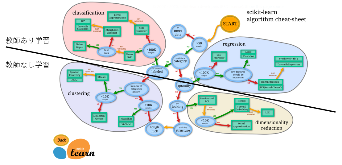
Supervised learning

--classification: Classification = The variable you want to predict is the class (example: "pass / fail", "sunny / cloudy / rain / snow") --Regression: Regression = The variable you want to predict is the value (Example: Weight "66.6kg, 32.3kg, ...")

Unsupervised learning

--clustering: Clustering (grouping of similar data) --Dimensionality reduction: Dimensionality reduction (many features => reduce to a few essential features, both principal component analysis)

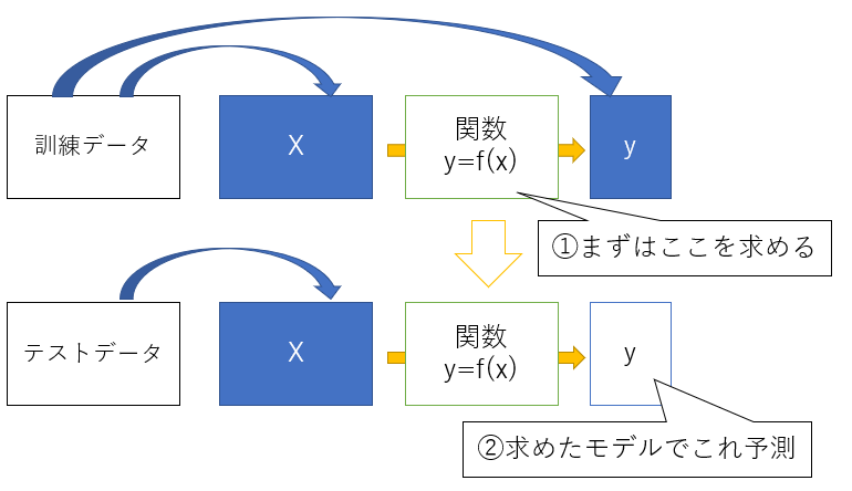
Supervised learning

A method of finding a model that predicts the objective variable (y) from the explanatory variable (or feature: X).

Overall picture of supervised learning model (Chapter 8 of the example book)

Roughly speaking, the following four.

1. Linear model
2. Decision tree
3. kNN (k-nearest neighbor method)
4. SVM (Support Vector Machine)

Each has a classification and regression model. 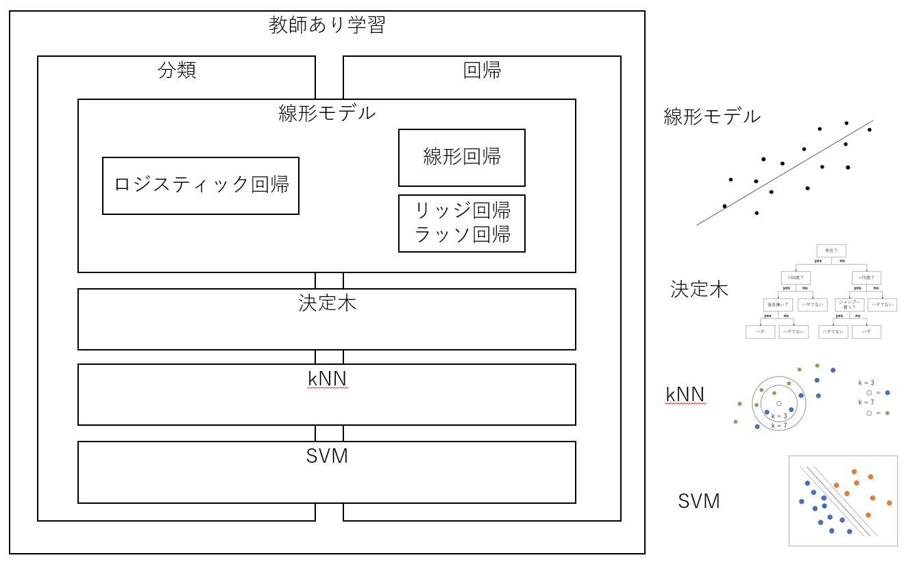The figure on the right is the point.

Details

The details of the model and the mathematical background are omitted because there are many other articles (← ~~ I can't explain it well yet ~~)

1. Linear model

image

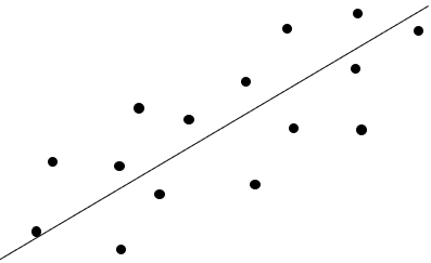
Since it is linear, it is an image of a first-order polynomial (y = ax + by + cz). It really looks like this.

y = w_0x_0+w_1x_1+w_2x_2+\cdots

There are multiple models even for the basic ones. Regression with regularization terms, or the name is so cool that I always forget which one.

Simple regression, multiple regression

Simple regression: One explanatory variable.

y = ax+b

Multiple regression: Multiple explanatory variables.

y = w_0x_0+w_1x_1+w_2x_2+\cdots

Find the optimum coefficient (weight) for each term by the least squares method (the sum of the squares of the "correct answer-predicted value" = the method of minimizing the penalty of how far away from the correct answer). You win if the following loss function is minimized.

loss = \sum_{i=1}^n(y_i-f(x_i))^2

Modeling

from sklearn.linear_model import LinearRegression
model = LinearRegression()

Parameters: Oh, I didn't set anything. ..

Lasso regression, ridge regression

The story of regularization. Regularization is, to put it simply, a method of preventing the model from becoming too complicated. I want to prevent a phenomenon (= overfitting) in which unknown data cannot be predicted in a good way because it adapts too much to training data. I want to improve generalization performance (prediction accuracy for unknown data such as test data). By adding a regularization term (which increases as the model becomes more complex) to the penalty, it is prevented from becoming more complex.

loss = \sum_{i=1}^n(y_i-f(x_i))^2+\lambda\sum_{j=1}^m|w_j|^q

** Lasso: q = 1 **: Regularization term (L1 norm) = Add sum (1st power) of weights ** Ridge: q = 2 **: Regularization term (L2 norm) = sum of squares of weights ~~ Roomba: Robot Vacuum Cleaner ~~ Involuntarily, I want to write "Aiueo".

By the way, I heard the following points from wind rumors, though it exceeds the contents of the book. ~~ I don't know. ~~

** Lasso ** sets the coefficient of unnecessary explanatory variables (features) to 0, so it seems to be convenient when you want to remove unnecessary parameters (sparse estimation). Oh, how do you use it properly with the dimension reduction of unsupervised learning? ?? ?? ** Ridge ** makes it possible to make good estimates even in situations where normal linear regression does not work due to multicollinearity (these coefficients are not determined to be good because they contain highly correlated features). It seems that they will do it.

By the way, if you combine the L1 norm and the L2 norm, Elastic Net! Because. ~~ I don't know. ~~

By the way, if you graph the regularization term (Lp norm), it looks like ** like this **. By the way, I like the figure in "Ridge Regression" of ** here **. (Hey, w from the top)

By the way, why can the coefficient (parameter) be set to 0 only in the case of Lasso ... The meaning of changing the parameter value is different. In the case of ** Ridge **, it is more effective to reduce the parameter with a large value as a penalty for the square of the parameter than to reduce the parameter with an originally small value (that's right). So, rather than moving a particular parameter closer to 0, it moves towards reducing another large parameter. Therefore, the coefficient is unlikely to be 0. In the case of ** Lasso **, it is the absolute value of the parameter, so regardless of the size of the original value, reducing the coefficient by 1 will reduce the penalty by 1. So you can easily reduce it to 0. Because. (That's true)

Modeling (Lasso)

from sklearn.linear_model import Lasso
model = Lasso(alpha=1.0, random_state=0)

Parameter: alpha (value of "λ (lambda)" in loss above, default = 1)

Modeling (Ridge)

from sklearn.linear_model import Ridge
model = Ridge(random_state=0)

Parameters: random_state

Logistic regression

This is the trick to solve the classification problem with a linear model. Binary classification can be done by using the sigmoid function. Multi-class classification only extends it to "one-to-other". It is easy to understand if it is a graph, but the first-order polynomial mentioned earlier will be included in the x part below. 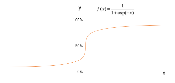Somehow, it seems that those with y of 50% or more should be classified as upper, and those with y of 50% or more should be classified as lower, but it is also important where to set this threshold (50%).

In the process of model learning, a loss function is used, which is defined so that the predicted value approaches the correct answer and the penalty increases when a predicted value far from the correct answer is given. If you can build the model so that the penalty is minimized (= if you can find a good coefficient), you win. The penalty (cross entropy error) looks like this. 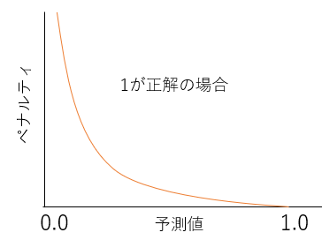If you want to make it a function (Tell me! Google teacher "y =-log x graph")

-log(Predicted value)

If 0 is the correct answer, flip the function horizontally. (Tell me! Google teacher "-log-(x-1) graph")

-log(-(Predicted value-1))

Modeling

from sklearn.linear_model import LogisticRegression
model = LogisticRegression()

Parameters: Oh, I didn't set anything. ..

2. Decision tree

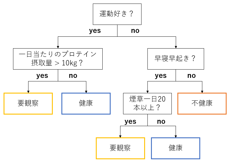
Easy pretreatment. (This time, pretreatment and details are omitted) No scaling required (no effect because the branching condition is related to the size of the value) No need to process missing values ​​(the missing values ​​are treated as special values)

I'll do my best to study from the base guys such as xgboost and LightGBM, which are often used in competitions. ~~ Only surface vine ~~

Teka, ** here ** Look, really.

Classification

See "Classification Tree" in the link, seriously.

Modeling

from sklearn.tree import DecisionTreeClassifier
model = DecisionTreeClassifier(criterion='entropy', max_depth=5, random_state=0)

Parameters:

• criterion : {“gini”, “entropy”}, default=”gini” --max_depth: Maximum depth of the tree

Regression

See "Regression Tree" in the link, seriously.

Modeling

from sklearn.tree import DecisionTreeRegressor
model = DecisionTreeRegressor()

Parameters: Oh, I didn't set anything. ..

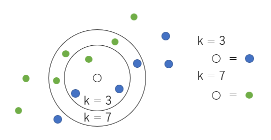
3. kNN (k-nearest neighbor method)

Majority vote by k with similar attributes Teka ** here ** Look at it. seriously. (Mushroom story, interesting)

Classification

Tell me what kind of mushrooms you have (see linked PDF)

Modeling

from sklearn.neighbors import KNeighborsClassifier
model = KNeighborsClassifier(n_neighbors=5)

Parameters: n_neighbors: k number

Regression

Tell me about the diameter of mushrooms (see linked PDF)

Modeling

from sklearn.neighbors import KNeighborsRegressor
model = KNeighborsRegressor(n_neighbors=5)

Parameters: n_neighbors: k number

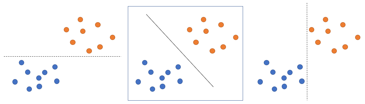
4. SVM (Support Vector Machine)

A method of drawing a border that identifies a category so that the margin is maximized. In the figure, it is neither left nor right, but in the middle.

Teka ** here ** Look at it. seriously.

Classification

The article above is just right.

Modeling 1

from sklearn.svm import LinearSVC
model = LinearSVC()

Parameters: That, nothing ... (ry

Modeling 2

from sklearn.svm import SVC
model = SVC(probability=True)

Parameters: --probability: Must be True to use the function predict_proba, which can get the probability of each classification class as a result of prediction, instead of the final determined classification class.

Regression

So ** here ** Look at it. seriously.

Modeling

from sklearn.svm import SVR
model = SVR()

Parameters: That, nothing ... (ry

Implementation

Process flow

1. Model creation (see each theory above)
2. Model training
3. Evaluation of the model

#The model can be anything. Here is multiple regression.
model = LinearRegression()
#Training
model.fit(X_train, y_train)
#Evaluation
print('train:', model.score(X_train, y_train))
print('test:', model.score(X_test, y_test))

About model.score

With a value between 0 and 1, the following is actually calculated. For ** classification **, accuracy For ** regression **, the coefficient of determination: R ^ 2

More big picture

import pandas as pd
from sklearn.datasets import load_iris
from sklearn.model_selection import train_test_split
from sklearn.linear_model import LogisticRegression

#Data load
iris = load_iris()

#Split test data
X_train, X_test, y_train, y_test = train_test_split(iris.data, iris.target, random_state=0)

#Model construction-evaluation
model = LogisticRegression()
model.fit(X_train, y_train)
print('train:', model.score(X_train, y_train))
print('test:', model.score(X_test, y_test))

result: train: 0.9821428571428571 test: 0.9736842105263158

Model comparison

import pandas as pd
from sklearn.datasets import load_iris
from sklearn.model_selection import train_test_split
from sklearn.linear_model import LogisticRegression
from sklearn.tree import DecisionTreeClassifier
from sklearn.neighbors import KNeighborsClassifier
from sklearn.svm import SVC

iris = load_iris()

X_train, X_test, y_train, y_test = train_test_split(iris.data, iris.target, random_state=0)

models = {
    'linear': LogisticRegression(),
    'tree': DecisionTreeClassifier(),
    'knn': KNeighborsClassifier(n_neighbors=3),
    'svm': SVC()
}

scores = {}

for name, model in models.items():
  #Model construction-evaluation
  model.fit(X_train, y_train)
  scores[(name, 'train')] = model.score(X_train, y_train)
  scores[(name, 'test')] = model.score(X_test, y_test)

pd.Series(scores).unstack()

result:

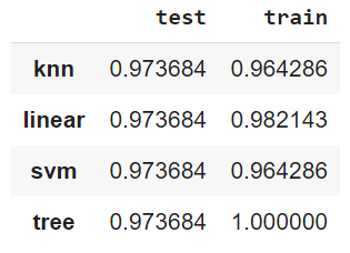
Summary

There are four models of supervised learning that I learned this time.

1. Linear model
2. Decision tree
3. kNN (k-nearest neighbor method)
4. SVM (Support Vector Machine)

Each has a model for regression and classification.

Impressions

It's pretty simple to organize in this way. Only the almost linear model in the manual, and the link collection (bitter smile). In the future, I think it's better to dig deeper if you feel like it, but it seems more fun to improve the score by using xgboost or LightGBM rather than chasing the details of the theory. I would like to make a note about unsupervised learning in Chapter 9 in the near future.