[PYTHON] Enjoy Coursera / Machine Learning materials twice
Lately, I am taking Coursera's Maechine Learning (Stanford University, by Andrew Ng). Of course, the explanation video is also useful, but what makes this course so good is the programming task that is given every time. It's just Matlab code, so I wanted to rewrite it to Python so that I could review it later. (Other people can see examples of the same efforts on the Internet.)
Here, I will introduce how to enjoy the teaching materials of "Coursera / Machine Learning" twice or three times (in Python). We also explain ** scipy.optimize.minimize () ** used for function minimization.
Cost function and its derivative
Many Machine Learning materials create a cost function and search for parameters that minimize it. Matlab uses fminunc () (or fmincg () provided in the task), but in Python ** scipy.optimize.minimize () ** supports a similar function.
First, prepare the cost function and its derivative by yourself. In the first task, the linear model, it is given by the following equation.
J(\theta) = \frac{1}{2m} \sum_{i=1}^{m} (h_{\theta}(x ^{(i)} ) -y ^{(i)}) ^2
\\
\frac{\partial J}{\partial \theta _j} = \frac{1}{m} \sum_{i=1}^{m}
(h_{\theta} (x^{(i)}) - y^{(i)} )x_j^{(i)}
$ h_ {\ theta} $ is the function assumed in modeling. (This time, a linear model is assumed.)
def compute_cost(theta, xmat, ymat):
    m = len(ymat)

    one_v = np.ones(len(xmat))
    xmat1 = np.column_stack((one_v, xmat)) # shape: m x 2
    ymat1 = ymat.reshape(len(ymat),1)      # shape: [m,] --> [m,1]
    theta1 = theta.reshape(len(theta),1)
    hx2y = np.dot(xmat1, theta1) - ymat1    # shape: m x 1
    j =  1. /2. /m * np.dot(hx2y.T, hx2y)  # shape: 1 x 1

    return j

def compute_grad(theta, xmat, ymat):
    j_grad = np.zeros(len(theta), dtype=float)

    m = len(ymat)
    one_v = np.ones(len(xmat))
    xmat1 = np.column_stack((one_v, xmat))
    ymat1 = ymat.reshape(m,1)      # shape: [m,] --> [m,1]
    theta1 = theta.reshape(len(theta),1)
    hx2y = np.dot(xmat1, theta1) - ymat1
    j_grad = 1. /m * np.dot(xmat1.T, hx2y)
    j_grad = j_grad.flatten()

    return j_grad
It is an implementation of such a function. Using these two functions as subordinate functions, the parameter (theta) search that minimizes the cost is performed by the gradient descent method. First, the following formula shown in Coursera is coded as it is and the calculation is performed.
Gradient descent equation:
\theta_i := \theta_j - \alpha \frac{1}{m} \sum_{i=1}^{m} (h_{\theta} (x^{(i)}) - y^{(i)}) x_{j}^{(i)} \ \ \ \ \ (simultaneously\ update\ \theta_j\ for\ all\ j)
def gradient_descent(theta, alpha, num_iters):
    global xmat, ymat

    m = len(ymat)      # number of train examples
    j_history = np.zeros(num_iters)
    #
    for iter in range(num_iters):
        xmat1 = xmat ; ymat1 = ymat
        delta_t = alpha * compute_grad(theta, xmat1, ymat1)
        theta = theta - delta_t
        # for DEBUG #
        j_history[iter] = compute_cost(theta, xmat, ymat)

    return theta, j_history
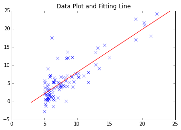
The simplest gradient descent method is as described above. Coursera / Machine Learning This is no problem for the first task. The found Fitting line is as follows.
However, considering the convergence of larger-scale data and complex data analysis and the correspondence to local minimum points, there may be cases where you want to use a module with a proven track record.
Try using scipy.optimize.minimize ()
Various functions are implemented in Scipy for optimization.
http://docs.scipy.org/doc/scipy/reference/optimize.html
This time, I decided to use ** scipy.optimize.minimize () **, which has the function of "minimizing the function that refers to the parameter". Excerpt from the documentation.
scipy.optimize.minimize (fun, x0, args=(), method=None, jac=None, hess=None, hessp=None, bounds=None, constraints=(), tol=None, callback=None, options=None)
parameters
- fun : callable Objective function.
- x0 : ndarray Initial guess.
- args : tuple, optional Extra arguments passed to the objective function and its derivatives (Jacobian, Hessian).
- method : str or callable, optional Type of solver. Should be one of -- ‘Nelder-Mead’ -- ‘Powell’ -- ‘CG’ -- ‘BFGS’ -- ‘Newton-CG’ -- ‘L-BFGS-B’ -- ‘TNC’ -- ‘COBYLA’ -- ‘SLSQP’ -- ‘dogleg’ -- ‘trust-ncg’ -- custom - a callable object If not given, chosen to be one of BFGS, L-BFGS-B, SLSQP
- jac : bool or callable, optional (Hereafter omitted)
It lists calculation methods that I haven't seen much, and it is encouraging even though I am not familiar with the contents. First, I tested it with a simple mathematical formula.
import scipy.optimize as spo
def fun1(x):
	ans = (x[0] - 1.5) ** 2 + (x[1] - 2.5) ** 2

	return ans

def fun1_grad(x):
	dx = np.zeros(2)
	dx[0] = 2 * x[0] - 3
	dx[1] = 2 * x[1] - 5

	return dx

x_init = np.array([1.0, 1.0])   # initial value

res1 = spo.minimize(fun1, x_init, method='BFGS', jac=fun1_grad, \
            options={'gtol': 1e-6, 'disp': True})
This gives us $ x = [1.5, 2.5] $ which minimizes $ f = (x_0 --1.5) ^ 2 + (x_1 --2.5) ^ 2 $. For Coursera's tasks, we did the following. First, prepare a wrapper for the cost function and derivative.
def compute_cost_sp(theta):
    global xmat, ymat
    j = compute_cost(theta, xmat, ymat)

    return j

def compute_grad_sp(theta):
    global xmat, ymat
    j_grad = compute_grad(theta, xmat, ymat)

    return j_grad
The purpose of this is to clarify that the parameter to be searched by omitting the arguments (xmat, ymat) is "theta". Call scipy.optimize.minimize () by passing a function or derivative that takes only "theta" as an argument. (I'm supposed to use global variables ...)
    theta_ini = np.zeros(2)
    res1 = spo.minimize(compute_cost_sp, theta_ini, method='BFGS', \
         jac=compute_grad_sp, options={'gtol': 1e-6, 'disp': True})
    print ' theta.processed =', res1.x
Actually, it is possible to pass the necessary data (xmat, ymat) with ** args ** without writing a wrapper, but I was conscious of clarifying the "adjustment parameters" here. The calculation results are as follows.
#Your own Gradient Descent(iteration =2000 times)
theta =     -3.788,      1.182
# scipy.optimize.minimize()Result of
Optimization terminated successfully.
         Current function value: 4.476971
         Iterations: 4
         Function evaluations: 6
         Gradient evaluations: 6
 theta.processed = [-3.89578088  1.19303364]
Try to be stochastic
From here, it is an advanced version that is not included in the task (it was done arbitrarily). I tried "trial" of Stochastic Gradient Descent, which is often used in deep learning.
def stochastic_g_d(theta, alpha, sample_ratio, num_iters):
    # calculate the number of sampling data (original size * sample_ratio)
    sample_num = int(len(ymat) * sample_ratio)

    m = len(ymat)      # number of train examples (total)
    n = np.size(xmat) / len(xmat)
    j_history = np.zeros(num_iters)

    for iter in range(num_iters):
        xs = np.zeros((sample_num, n)) ; ys = np.zeros(sample_num)

        for i in range(sample_num):
            myrnd = np.random.randint(m)
            xs[i,:] = xmat[myrnd,]
            ys[i]   = ymat[myrnd]

        delta_t = alpha * compute_grad(theta, xs, ys)
        theta = theta - delta_t
        j_history[iter] = compute_cost(theta, xmat, ymat)

    return theta, j_history
In the above code, the process from sampling to minimization of Train Data was done by my own code, but of course it is also possible to find the solution with scipy.optimize.minimize () after sampling Train Data.
For a detailed explanation of S.G.D. (Stochastic Gradient Descent), refer to the reference (web article). The "liver" is to sample the data used to calculate the cost function and derivative. Since the number of train data this time is small, less than 100, there is no need to use S.G.D., but in the case of handling large-scale data, the calculation efficiency can be greatly improved.
The following is a drawing of the Learning Curve. (Horizontal axis: number of loop calculations, vertical axis: cost, normal gradient descent method and stochastic gradient descent method.)
Gradient Descent Method (reference)

Stochastic Gradient Descent (sampling/whole data= 0.3)

It's fun to be able to expand the scope by yourself while doing tasks with Cousera. I'm still in the middle of taking Machine Learning this time, but what should I take next to Machine Learning? I'm thinking about various things. Recently, the number of paid courses "Specialization" has increased, but some of the free courses are also of interest. (It takes a lot of time, but ...)
References
- Cousera, Machine Learning (Stanford University) (A programming task manual / PDF will be distributed every week.)
- Scipy Documentation http://docs.scipy.org/doc/scipy/reference/optimize.html
- Theano, Deep Learning Tutorial http://deeplearning.net/tutorial/ --Qiita: [Update] Explain what the stochastic gradient descent method is by running it in Python http://qiita.com/kenmatsu4/items/d282054ddedbd68fecb0 / d282054ddedbd68fecb0) -(Series) Machine Learning Let's get started, Part 16 Gradient method for optimization http://gihyo.jp/dev/serial/01/machine-learning/0016
Recommended Posts