[PYTHON] Variational Autoencoder Thorough explanation
This article introduces one of the deep learning models, the Variational Autoencoder (VAE). I'm trying using Chainer as a deep learning framework.
With VAE, you can create images like this. VAE is one of the generative models by deep learning, and it is possible to generate data similar to the training data set by capturing its characteristics based on the training data. Below is an animation of the data generated by VAE. Please see the text for details.

The Python code for this article can be found at here.
1. What is Variational Autoencoder?
First, I would like to explain what VAE is, but before that, I would like to touch on ordinary autoencoders.
1-1. Normal autoencoder
What is an autoencoder?
- One of unsupervised learning. Therefore, the input data at the time of learning is only training data, and teacher data is not used.
- A neural network for acquiring features that represent data.
It has such characteristics. Taking MNIST as an example, it is a neural network that puts an image of 28x28 numbers and outputs the same image. It is an image of the figure below. The neural network that converts the input data $ X $ to the latent variable $ z $ is called an Encoder. (It is named Encoder because the input data can be regarded as encoded.) At this time, if the dimension of $ z $ is smaller than the input $ X $, it can also be regarded as dimension reduction. Conversely, a neural network that restores the original image using the latent variable $ z $ as input is called a Decoder.

When the case where the neural network has one layer is expressed by a mathematical formula,
\hat{x}(x) = \hat{f}(\hat{W} f(Wx+b)+\hat{b})
is. Loss at this time
Loss = \sum_{n=1}^N \|x_n - \hat{x}(x_n) \|^2
will do. This is called Reconstruction Error. It can be learned by updating the weight by the error back propagation method so that it is as close as possible to the input data.
1-2. Variational Autoencoder(VAE)
The big difference is that VAE assumes a probability distribution for this latent variable $ z $, usually $ z \ sim N (0, 1) $. With a normal autoencoder, I'm pushing data into the latent variable $ z $, but I'm not sure what the structure is. VAE makes it possible to push the latent variable $ z $ into a structure called a probability distribution.
The image is below.

I'm not sure yet. If you look at what you actually run the program, you will get a little image.
First, let's compare the input and output. (This was learned by setting the dimension of $ z $ to 20.) It's a little vague, but the original shape is almost restored. Since MNIST is originally 784-dimensional data, it can be said that most of the essential features could be incorporated into the 20-dimensional reduced dimension.

Next, let's see the behavior only in the Encoder part. Assuming that there is an Encoder that has already been trained, put a dataset of training data in it and drop it into a latent variable. The dimension of $ z $ is two-dimensional so that it can be visualized. You can see that the MNIST dataset of training data is scattered on a circle that follows a two-dimensional normal distribution. Also, although this is a miso, it can be seen that data with the same class label are gathered in close proximity despite unsupervised learning without teacher data. This is because VAE is designed so that $ z $ follows a normal distribution and incorporates random numbers that follow a normal distribution during learning, so this random number blur has the effect of bringing similar shapes closer together. In other words, even if you input the same image, $ z $ will be plotted at a slightly different position each time, and the image generated by Decoder from that $ z $ will be the same as the input image. The position where the numbers are plotted in text in the scatter plot below is in the center of each label.

Now, what if we try to generate data by shifting the data little by little along the space of the latent variable from "0" to "7"?

The animation below is the result.
t\cdot z_0 + (1-t)\cdot z_7, \ \ 0\leq t \leq 1
As shown, the MNIST image is generated by Decoder with the input of $ t $ moved from 0 to 1. You can see how it starts from 0 and goes through the numbers between 0-6-2-8-9-4-7 and 7: wink: These are N (0), not the training data itself. , 1) The miso is that the image is generated by VAE mapped above.

The following is the one displayed frame by frame.

The figure below shows $ -2 \ leq z_1 \ leq 2, \ -2 \ leq z_2 \ leq 2 $ cut out from the two-dimensional space of $ z $, input to the Decoder, and the corresponding output image is displayed. Become. The red line is the trajectory of the previous movement.

From the training data, it can be seen that the positional relationship is almost the same as the map of $ z $ generated by Encoder. On the contrary, the place where the probability (density) is very low from the viewpoint of N (0, 1) is far from the original data set, so the corresponding generated image is broken in the form of numbers. It can be said that this correctly represents the structure of the probability distribution of data generation.

It is a diagram showing all the situations that start from 0 to 9 and reach 0 to 9 each. This example increases the dimension of the latent variable to 20. So, unlike before, the number of numbers that go through on the way will decrease. The high dimension makes it more expressive.
1-3. Manifold hypothesis
One of the features of Deep Learning is that it can combine task learning and expression learning. High-dimensional data such as images are actually distributed only in a small part of the high-dimensional data, and meaningful data (data that captures the essence of training data) is in the high-dimensional data. There is a manifold hypothesis that is considered to be locally solidified. I think the example of Swiss roll data below is easy to understand. The data is distributed in three dimensions, but the data is fairly locally biased, and you can see that most of the data can actually be represented in two dimensions. There is a gap with no data between the rolls. Therefore, the data with short distances in three dimensions are not always similar, and it is more likely that similar data will be found by considering the distance by moving in the direction along the phase. So it's better to open it in two dimensions and measure the distance.
 [Swiss roll as a two-dimensional manifold in three dimensions]
 [When you expand the Swiss roll in two dimensions, it looks like this]
Returning to the MNIST VAE from the Swiss Roll, it is the VAE that captures this manifold and pushes the data from the 784-dimensional MNIST image data dimension to the latent variable $ z \ sim N (0, 1) $. Please also refer to [7] for expression learning and manifold hypothesis.
2. Implementation with Chainer
I will explain using a customized version based on Chainer Official Example. Encoder and Decoder are modeled using 3-layer MLP (Multi Layer Perceptron).
The Computation Graph output by Chainer prior to the code is shown below. You can see that the MLP part of the three layers of Encoder and Decoder and the use of Gaussian, that is, a random number that follows a normal distribution, to generate the latent variable $ z $. Encoder expresses $ z $ by outputting the parameters $ \ mu $ and $ \ sigma ^ 2 $ of this normal distribution.

# Reference: https://jmetzen.github.io/2015-11-27/vae.html
class Xavier(initializer.Initializer):
    """
    Xavier initializaer
    Reference:
    * https://jmetzen.github.io/2015-11-27/vae.html
    * https://stackoverflow.com/questions/33640581/how-to-do-xavier-initialization-on-tensorflow
    """
    def __init__(self, fan_in, fan_out, constant=1, dtype=None):
        self.fan_in = fan_in
        self.fan_out = fan_out
        self.high = constant*np.sqrt(6.0/(fan_in + fan_out))
        self.low = -self.high
        super(Xavier, self).__init__(dtype)

    def __call__(self, array):
        xp = cuda.get_array_module(array)
        args = {'low': self.low, 'high': self.high, 'size': array.shape}
        if xp is not np:
            # Only CuPy supports dtype option
            if self.dtype == np.float32 or self.dtype == np.float16:
                # float16 is not supported in cuRAND
                args['dtype'] = np.float32
        array[...] = xp.random.uniform(**args)


# Original implementation: https://github.com/chainer/chainer/tree/master/examples/vae
class VAE(chainer.Chain):
    """Variational AutoEncoder"""

    def __init__(self, n_in, n_latent, n_h, act_func=F.tanh):
        super(VAE, self).__init__()
        self.act_func = act_func
        with self.init_scope():
            # encoder
            self.le1        = L.Linear(n_in, n_h,      initialW=Xavier(n_in, n_h))
            self.le2        = L.Linear(n_h,  n_h,      initialW=Xavier(n_h, n_h))
            self.le3_mu     = L.Linear(n_h,  n_latent, initialW=Xavier(n_h,  n_latent))
            self.le3_ln_var = L.Linear(n_h,  n_latent, initialW=Xavier(n_h,  n_latent))

            # decoder
            self.ld1 = L.Linear(n_latent, n_h, initialW=Xavier(n_latent, n_h))
            self.ld2 = L.Linear(n_h,      n_h, initialW=Xavier(n_h, n_h))
            self.ld3 = L.Linear(n_h,      n_in,initialW=Xavier(n_h, n_in))

    def __call__(self, x, sigmoid=True):
        """ AutoEncoder """
        return self.decode(self.encode(x)[0], sigmoid)

    def encode(self, x):
        if type(x) != chainer.variable.Variable:
            x = chainer.Variable(x)
        x.name = "x"
        h1 = self.act_func(self.le1(x))
        h1.name = "enc_h1"
        h2 = self.act_func(self.le2(h1))
        h2.name = "enc_h2"
        mu = self.le3_mu(h2)
        mu.name = "z_mu"
        ln_var = self.le3_ln_var(h2)  # ln_var = log(sigma**2)
        ln_var.name = "z_ln_var"
        return mu, ln_var

    def decode(self, z, sigmoid=True):
        h1 = self.act_func(self.ld1(z))
        h1.name = "dec_h1"
        h2 = self.act_func(self.ld2(h1))
        h2.name = "dec_h2"
        h3 = self.ld3(h2)
        h3.name = "dec_h3"
        if sigmoid:
            return F.sigmoid(h3)
        else:
            return h3

    def get_loss_func(self, C=1.0, k=1):
        """Get loss function of VAE.

        The loss value is equal to ELBO (Evidence Lower Bound)
        multiplied by -1.

        Args:
            C (int): Usually this is 1.0. Can be changed to control the
                second term of ELBO bound, which works as regularization.
            k (int): Number of Monte Carlo samples used in encoded vector.
        """
        def lf(x):
            mu, ln_var = self.encode(x)
            batchsize = len(mu.data)
            # reconstruction error
            rec_loss = 0
            for l in six.moves.range(k):
                z = F.gaussian(mu, ln_var)
                z.name = "z"
                rec_loss += F.bernoulli_nll(x, self.decode(z, sigmoid=False)) / (k * batchsize)
            self.rec_loss = rec_loss
            self.rec_loss.name = "reconstruction error"
            self.latent_loss = C * gaussian_kl_divergence(mu, ln_var) / batchsize
            self.latent_loss.name = "latent loss"
            self.loss = self.rec_loss + self.latent_loss
            self.loss.name = "loss"
            return self.loss
        return lf
3. Theoretical overview of VAE
The purpose of the generative model is to estimate the distribution of data, $ p (X) $. In the words of PRML, it is as follows.
The approach of modeling not only the distribution of the output but also the distribution of the input, either yin or yang, is called the ** Generative model ** because sampling from the model can generate artificial data in the input space. " PRML Volume 1 p42)
When considering images, $ X $ is usually very high-dimensional data. Since this article targets MNIST, it is 784-dimensional data. As introduced in the previous section, there are very few places in this higher dimension where the data actually exists, so we can capture it well and the latent variable $ z of the lower dimension factor (for example, 10th dimension). Consider expressing it with $. In other words, we are trying to build a correspondence between high-dimensional data $ X $ and low-dimensional data $ z $ and use it well. VAE trains this latent variable $ z $ to be distributed as a normal distribution and estimates $ p (X) $. $ p (X) $ is sometimes referred to as Evidence.
here,
- $ p (\ cdot) $: Probabilistic model
- $ z $: Latent variable
- $ X $: Data
will do. Given that this probability distribution has parameters, the maximum likelihood method for $ p (X) $ can be used to find the parameter for $ p (X) $ that best represents $ X $. In VAE, a neural network is used as a part of the elements that make up this probability distribution, and its parameters are obtained by the error back propagation method and the stochastic gradient descent method.
A graphical model of the relationship between the latent variable $ z $ and the data $ X $ looks like this.

The neural network that associates the data $ X $ with the latent variable $ z $ is called an Encoder. If you think about the analogy of image file compression like so-called jpeg, you can see why it is called Encoder.

Conversely, Decoder is a neural network that restores data $ X $ from a latent variable $ z $.

From the above, the VAE consisting of the Encoder, Decoder, and two neural networks can be modeled as follows. $ \ phi $ is the Encoder parameter and $ \ theta $ is the Decoder parameter. The point is that the Encoder does not generate $ z $ directly, but rather the parameters $ \ mu, \ sigma $ of the normal distribution that $ z $ follows, as shown below.

We have determined that the model $ p (X) $ we want to estimate is a model consisting of two neural networks as described above. The rest is the procedure to find the parameters that fit the data. Considering the steps below, we can see that we should find the parameter that maximizes the variational lower –bound $ L (X, z) $ (described later). The variational lower limit is sometimes called ELBO (Evidence Lower BOund).
** Steps of thinking to find parameters **
- Find the neural network parameters $ \ theta, \ phi $ that maximize the likelihood of $ p (X) $ by the maximum likelihood method.
- Target the log-likelihood $ \ log p (X) $ for ease of use.
- Since it is difficult to handle the integral by maximizing $ \ log p (X) $ as it is, logarithmic likelihood is achieved by maximizing the variational lower limit $ L (X, z) $ and suppressing it from the bottom. Find the parameter that maximizes the degree.
What is this variational lower limit? This is calculated as follows.
 Please also refer to [here](http://qiita.com/kenmatsu4/items/26d098a4048f84bf85fb) for Jensen's inequality.
Due to the inequality sign, $ L (X, z) $ represents the lower limit of $ \ log p (X) $, and there is a gap as represented by the "?" In the figure below.

Log-likelihood to find this "?"

In the last equation, it is greater than or equal to 0 because Kullback-Leibler divergence is always greater than or equal to 0.

Therefore, the lower limit of variation is

have become. Since the first term is a fixed value and the second term is a parameter-dependent item, the target "maximization of the variational lower limit" is Kullback-Leibler divergence.
This Kullback-Leibler Divergence

Substitute this into the variational lower bound equation.

Now we know that the variational lower limit can be represented by two terms.

The second item is
            mu, ln_var = self.encode(x)
            batchsize = len(mu.data)
            # reconstruction error
            rec_loss = 0
            for l in six.moves.range(k):
                z = F.gaussian(mu, ln_var)
                z.name = "z"
                rec_loss += F.bernoulli_nll(x, self.decode(z, sigmoid=False)) / (k * batchsize)
Assume that $ p_ {\ theta} (X | z) $ follows a multivariate Bernoulli distribution (from [3] C.1 Bernoulli MLP as decoder) [F.bernoulli_nll](https://docs.chainer.org/ The loss is calculated with en / stable / reference / generated / chainer.functions.bernoulli_nll.html # chainer.functions.bernoulli_nll). In other words, assuming that each pixel takes a value between 0 and 1, it is considered that the output of VAE and the input image have cross entropy. This loss is called Reconstruction Error.

First item
self.latent_loss = C * gaussian_kl_divergence(mu, ln_var) / batchsize
The core part of'gaussian_kl_divergence'is as follows.
    var = exponential.exp(ln_var)
    mean_square = mean * mean
    loss = (mean_square + var - ln_var - 1) * 0.5
It calculates the Kullback-Leibler divergence when following a normal distribution. (See [3] APPENDIX B)

(For the derivation of Kullback Leibler Divergence in the case of normal distribution, please refer to the commentary article written in here.)
Now you can calculate what you want to maximize. Since the learning of the neural network is performed with the value of minimizing the loss, the parameters $ \ theta and \ phi $ are optimized by multiplying this variational lower limit by a minus as the loss function.
Reparameterization Trick
The last problem is that with the above structure, there is a probability distribution of $ z \ sim N (\ mu (X), \ sigma (X)) $ in between, so the error back propagation method is used. It will not be possible to apply below. A technique called Reparameterization Trick is used to solve this. Instead of dealing directly with $ z \ sim N (\ mu (X), \ sigma (X)) $, generate noise at $ \ varepsilon \ sim N (0, I) $ and $ z = \ mu By connecting in the form of (X) + \ varepsilon * \ sigma (X) $, VAE is constructed as shown in the figure below, avoiding random variables and following the blue arrow in reverse, and applying the error back propagation method. It is something to do.

In terms of Chainer code, the following is applicable.
            mu, ln_var = self.encode(x)
            batchsize = len(mu.data)
            # reconstruction error
            rec_loss = 0
            for l in six.moves.range(k):
                z = F.gaussian(mu, ln_var)
bonus
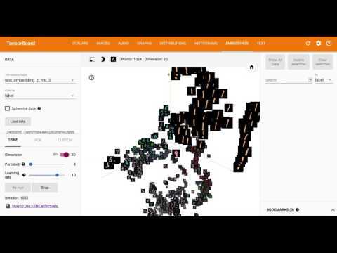
Using Embedding, one of the functions of TensorFlow's Tensorboard, the 20-dimensional latent variable $ z $ is visualized by reducing it in 3D and 2D with T-SNE.
reference
[1] Python code for this article https://github.com/matsuken92/Qiita_Contents/tree/master/chainer-vae
[2] Tutorial on Variational Autoencoders https://arxiv.org/abs/1606.05908
[3] Auto-Encoding Variational Bayes(Diederik P Kingma, Max Welling) https://arxiv.org/abs/1312.6114
[4] Variational Bayesian method for natural language processing (Daichi Mochihashi) http://chasen.org/~daiti-m/paper/vb-nlp-tutorial.pdf
[5] Variational Auto Encoder (Sho Tatsuno) that even cats can understand https://www.slideshare.net/ssusere55c63/variational-autoencoder-64515581
[6] Deep Learning (Seiya Tokui) of generative model https://www.slideshare.net/beam2d/learning-generator
[7] IIBMP2016 Feature learning with deep generative model https://www.slideshare.net/pfi/iibmp2016-okanohara-deep-generative-models-for-representation-learning
[8] Variational AutoEncoder https://www.slideshare.net/KazukiNitta/variational-autoencoder-68705109
[9] Deep Learning Chapter 17 The Manifold Perspective on Representation Learning http://www.deeplearningbook.org/version-2015-10-03/contents/manifolds.html