[PYTHON] Gold needle for when it becomes a stone by looking at the formula of image processing
Image processing is difficult. Looking at Instagram's beautiful filters, Google's Photo Sphere, and those services, the images look interesting! An image processing book that opened with excitement. We had no choice but to petrify the mathematical formulas listed there, but what else is left to the voice whispered in our ears, "OpenCV will do the difficult things, right?" I could have done it.
I hope that this article will show the way (in terms of items, gold needles) to those who want to overcome those days when they had to petrify and understand the basic theory while using OpenCV. think. The scope of coverage is in Chapter 2 of Practical Computer Vision, which is the basis of all processing. Equivalent). In addition, since this article itself is written while being understood by me as a beginner, I would appreciate it if advanced image processing adventurers could point out any mistakes.
What are the feature points of the image?
Why can humans assemble jigsaw puzzles? Thinking about it, we can think of it as understanding the characteristics of each piece of the puzzle, finding similar and continuous characteristics, and connecting them together. Similarly, you can combine multiple photos into a panoramic photo because you find and connect common features between the photos.
 CS231M Mobile Computer Vision Class,Lecture5, Stitching + Blending, p4~
If you think about these "feature points" more and more simply, you can finally summarize them into the following three points.

- edge: There is a boundary where the difference can be recognized
- corner: The point where edges are concentrated
- flat: Neither edge nor corner, the point that no feature can be recognized
And, considering the composition of panoramic photos as described above, it is necessary to follow the following rules when finding this "feature point".
- Reproducibility: A feature point is always recognized as a feature point
- Distinguishability: One feature point can be identified as distinctly different from another feature point
Regarding reproducibility, for example, if the feature points that are recognized when the angle at which the photograph is taken changes drastically, the process of connecting the feature points will break down.

Therefore, it is better to be able to recognize robust feature points ** that do not change with the angle or magnification of the image.
With regard to distinctiveness, if the recognized feature points cannot be uniquely identified, it will be difficult to know which one to match.

Therefore, it is important to have a representation method that allows each feature point to be uniquely identified.
This is exactly what is required for Feature Detection and Feature Description. In other words, detecting "a robust feature point that does not change with the angle or magnification of the image" (Feature Detection) and expressing it with a "uniquely identifiable expression method" (Feature Description) is the image. It is the goal of recognizing feature points.
Now, let's look at the detection of feature points and the expression method of feature points in order.
Feature Detection
The procedure for detecting feature points is generally "detecting edges" and then "detecting corners" where edges are concentrated.
edge detection
Specifically, the edge is the "point where the brightness changes significantly". As a simple example, consider an image of a black tile with a white circle. If you plot the brightness on the red line drawn from the side as shown below along the coordinate axes, you should get a graph in which the brightness jumps in the white circle in the middle.

Here, what we want to detect is the edge, that is, the point on the graph that changes significantly from dark-> bright, bright-> dark. In order to know the degree of change at a certain point, let's calculate the rate of change from the values of the points before and after that point.
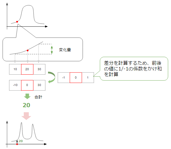
Then, as shown in the above figure, you can get a graph in which the rate of change is increasing at the point where the change is large, that is, the part corresponding to the edge (the amount of change has +-, but here the absolute value is plotted. Please think). Right now, we are thinking about the amount of change in the horizontal direction of the figure, but the same can be said for the vertical direction.
Ultimately, it seems that edge can be detected by summing the amount of change in both the horizontal and vertical directions (usually the square root of the sum of squares) and collecting points whose value is larger than a certain threshold.
This is the basic idea of edge detection, and although edge detection is possible with this alone, there are some techniques for more accurate detection, so let's take a look at it.
Smoothing
This is a method that considers the peripheral part when calculating the amount of change. Roughly speaking, it's like taking an average. By averaging, the change in value can be smoothed (smoothing), and as a result, smoothly connected edges can be detected.
The figure below shows how the amount of change in the horizontal direction is calculated by taking into account the amount of change at adjacent points. Smoothing is achieved by summing a total of three changes.
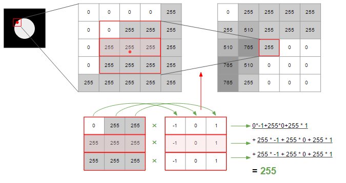
In the above figure, in order to calculate the amount of change, it is calculated using a matrix containing the value of -1/0/1 of 3 * 3. The matrix and processing for calculating such changes are called ** filters **.
There are various types of this filter, and the one used in the above figure is the Prewitt filter. Sobel filters focus more on what is adjacent to the center than Prewitt, and Gaussian uses a function of normal distribution to allow the center to be the apex and the coefficients to be gently multiplied toward the edges. The Canny method, which is often used to detect edges, is a method that uses this Gaussian filter.

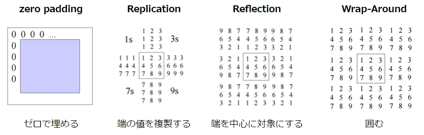
Note that it is necessary to perform interpolation for the edge of the image because there are no adjacent points. There are the following methods for this interpolation method.
 CSE/EE486 Computer Vision I, Lecture3, p26~
That's all for edge detection. I will summarize the contents so far.
- To detect edge, use the amount of change in brightness in the image as a clue.
- The amount of change can be taken in two directions, the horizontal direction and the vertical direction. The square root of the sum of squares of this value is used as the amount of change, and this is called Magnitude.
- Edge can be detected by determining edge when Magnitude exceeds a certain threshold.
- When calculating the amount of change, smoothing is generally performed. This is to improve the detection accuracy by adding the amount of change in the surroundings.
- Filters define the scope of this "periphery" and the weighting for it, and there are various types.
Corner detection
Next is the detection of corner. Here, we will explain the Harris Corner Detector, which is often used for corner detection. This is a method that makes good use of the characteristics of the matrix, and intuitively gives an image close to principal component analysis.

I will leave the detailed explanation of principal component analysis to other articles, but the following two points are important.
- Find indicators that can explain the direction of data spread. This corresponds to the eigenvectors of the matrix.
- The eigenvalues obtained as a result of the calculation represent the explanatory power of the index.
Applying this to Harris, the "data" is, of course, a summary of the amount of change in each of the horizontal and vertical directions at a certain point. Then, from the explanation of principal component analysis above, it can be inferred as follows.
- The eigenvector represents the "direction in which the amount of change spreads", that is, the direction of the edge.
- When the eigenvalue is large, it means that "the ability to explain the amount of change is high", that is, the strength of the edge.
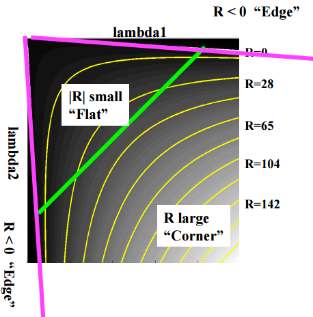
This makes it possible to detect edges first, and if there are "multiple eigenvectors with large eigenvalues", then it means that there are multiple edges, that is, corners. Assuming that the eigenvalues are $ \ lambda1 $ and $ \ lambda2 $, respectively, they can be classified as follows according to the size of the values.
 CSE/EE486 Computer Vision I, Lecture 06, Corner Detection, p19
I will also explain the formula. First, a point $ I (x, y) $ on the image $ I $ and a point $ I (x + u, y + v) moved by $ u $ in the $ x $ direction and $ v $ in the $ y $ direction. If the amount of change between) $ is $ E (u, v) $, the formula can be expressed as follows.
$ w (x, y) $ is a window function, which is a filter (Gaussian). The image is that the amount of change is $ [I (x + u, y + v) --I (x, y)] ^ 2 $, and this is smoothed with $ w (x, y) $ to calculate the amount of change. is. Approximating this formula using Taylor expansion is as follows (expansion formula is omitted. If you are interested, please refer to the lecture material linked above).
E(u, v) \simeq [u, v] M \begin{bmatrix} u \\ v \end{bmatrix}
Where $ M $ is:
M = \sum_{x, y} w(x, y) \begin{bmatrix} I_X^2 & I_x I_y \\ I_x I_y & I_y ^2 \end{bmatrix}
$ I_x $ and $ I_y $ are the differences on the x-axis and y-axis, respectively, and the square of $ [I_x, I_y] $ gives the above matrix part. What you are doing is the same as $ [I (x + u, y + v) --I (x, y)] ^ 2 $ in the above formula. And this is the "matrix that describes the amount of change", and by decomposing this into singular values, it is possible to judge the edge and corner as described at the beginning.
However, calculating the eigenvalues is a lot of work, so try not to calculate them where you don't need them. The following indicators are used for this purpose.
R = det M -k(trace M)^2
det M = \lambda1 \lambda2
trace M = \lambda1 + \lambda2
$ k $ is a constant, about 0.04 ~ 0.06. It can be classified as follows according to the value of R.
- Large R: corner
- Small R: flat
- R < 0: edge
The figure is as follows.
 CSE/EE486 Computer Vision I, Lecture 06, Corner Detection, p22
Now you can detect the corner quickly. Here is a summary of corner detection.
- corner can be defined as a place where multiple edges gather
- The direction of the edge can be found from the eigenvector of the matrix that summarizes the amount of change, and the magnitude of the amount of change (edge-likeness) can be found from the magnitude of the eigenvalue.
- Edge, corner, and flat can be determined based on the values of the two eigenvalues.
- Since the calculation of eigenvalues is troublesome, use the judgment formula to simplify the calculation.
Since Harris considers the eigenvectors that are the orientation of the edge, it is robust against the tilt of the image. However, it is not robust when it comes to scale. This is because the corners become looser as you expand, making it harder to distinguish the edges.
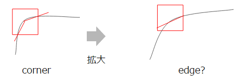
FAST is a devised method to overcome this. I will omit the details, but it is a method to recognize a series of n points darker or brighter than the center point. This is literally a FAST technique and is robust against rotation and expansion.
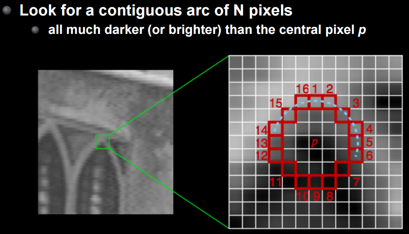 CS231M Mobile Computer Vision Class,Lecture5, Stitching + Blending, p24
Feature Description
The feature points can now be detected. Next time, I would like to be able to match images by creating a unique feature expression and Feature Description using the feature points.
As I mentioned a little, the following three characteristics are desirable for this Feature Description.
- Translation: Robust for image slides
- Rotation: Robust against image rotation
- Scaling: Robust for image scaling
Since Translation simply changes its position, it is relatively easy to deal with, and as mentioned in Harris in the previous section, Rotation is also quite good. However, it is difficult to support Scaling. As you can see from the figure below, the information in the image changes significantly depending on the magnification.
 CSE/EE486 Computer Vision I, Lecture 31, Object Recognition : SIFT Keys, p31
In the first place, if you expand it, it is obvious that the information will be lost if you do not expand the matching range accordingly. This is because the area that fits in the same range changes.

In other words, it is necessary to consider the scale to satisfy the above three characteristics. In Harris, only "direction" and "strength" were used from the eigenvectors and eigenvalues, but here we add "scale", that is, what enlargement value is obtained. The image looks like the following.

The SIFT method enables the detection and description of feature points that take this scale into consideration.
SIFT (Scale Invariant Feature Transform)
The heart of SIFT is the extraction of feature points for each scale. The method used for this is LoG / DoG. Log is an abbreviation of Laplacian of Gaussian, and the point with the largest amount of change in the image smoothed by the Gaussian filter is obtained by the second derivative (= Laplacian). Since Gaussian is as described in Smoothing, I will briefly explain why the point with the maximum amount of change is obtained by the second derivative (= Laplacian).

Think of differentiation as simply finding the amount of change at a certain point. Then you can see the following.
- First derivative: Represents the amount of change with respect to the original function = The vertex represents the point where the amount of change is maximum (minimum)
- Second derivative: A change in the direction of change occurs near the apex of the first derivative, which represents the change in the amount of change. The apex of the first derivative is equal to the zero-crossing point.
In other words, the point where $ I (x)'' = 0 $ is raised as the point with the largest amount of change and the feature point. The filter equivalent to applying this second derivative is called the "Laplacian filter", and the closer the value is to 0, the higher the possibility of feature points.
- However, it is not possible to distinguish between 0 (= no change) points and vertices at the stage of the first derivative only by the second derivative, so it is necessary to check at the same time whether the value of the first derivative is sufficiently large. As you can see from this, it is very vulnerable to noise.
Then, returning to LoG, as the name suggests, this is a method of smoothing with a Gaussian filter and then finding the point with the maximum amount of change = feature point with a Laplacian filter. And since LoG uses a Gaussian filter, you can adjust its $ \ sigma $ (variance). The larger $ \ sigma $ is, the stronger the smoothing will be, so it will only be possible to detect where points with large changes are gathered. This is the other way around, and as you may have noticed, it plays the same role as just manipulating the magnification.


CSE/EE486 Computer Vision I, Lecture 11, LoG Edge and Blob Finding, p19
SIFT detects feature points by preparing multiple hierarchies adjusted for this $ \ sigma $ (scale space). The following is the figure.

Here, in order to simplify the calculation of LoG, the approximation is performed by the difference between the two layers with different $ \ sigma $. This is the DoG (Difference of Gaussian). The found feature points are compared with the front and back scales to see if they are robust against the scale (compared with 8 points around and 9 points each on the front and back scales, for a total of 26 points).
Now you can see the robust features on the scale. The rest is the "strength" and "direction" of the amount of change at this feature point, which is obtained from the amount of change and its angle.

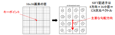
Here, SIFT considers not only a single feature point, but also 16 * 16 cells centered on it (the size of this "mass" is called [bin size](http: // www). .vlfeat.org/api/sift.html)).
 Semantic multimedia processing A2, p4
Divide it into 4x4 areas, and create a histogram with the vertical axis representing the amount of change (magitude of the amount of change) and the horizontal axis oriented (= the angle of the gradient of the amount of change).
 CSE/EE486 Computer Vision I, Lecture 31, Object Recognition : SIFT Keys, p24
The above figure is summarized from 0 to 36 (corresponding to 360 degrees), but finally it is summarized in 8 directions. Then, a vector is created in which each 4 * 4 window has elements in 8 directions. This 128-dimensional vector is the SIFT Vector, which is a feature point description with three characteristics: it is robust to "scale" and "strength" and "direction" are known.
By using this SIFT Vector, it becomes possible to match feature points with extremely high accuracy.
Evolution of feature point detection method
The methods for detecting and describing feature points listed above are evolving year by year. The following is the evolution of the method before and after the appearance of SIFT. You can see the process of obtaining features that are robust against rotation and scale.
 MIRU2013 Tutorial: SIFT and subsequent approaches, p5
This is the evolution after SIFT. A technique called SURF, which accelerates SIFT, is also often used. Both SIFT and SURF are patented **. SIFT patent expired on March 6, 2020, and OpenCV also [out of NON FREE](https://github.com/ opencv / opencv_contrib / pull / 2449), but there is still a patent fee for using SURF. Therefore, I have explained so far, but it seems that ORB and AKAZE added in OpenCV 3.0 are good for actual use. Nothing is faster than SIFT / SURF.
 MIRU2013 Tutorial: SIFT and subsequent approaches, p93
If you understand the basic methods introduced this time, it will be easier to understand what has been improved when new methods appear in the future.
Feature point matching
The detected feature points can be used for various purposes. As a typical example, I would like to introduce the method used for image matching.
First, when matching images, the basic flow is to cut out the area around the feature point to be compared (this cut out is called a patch) and check if it is also in the other image. Become. There are two types of how to use this patch:
- Template-based: Check the other image for a match with the patch
- Feature-based: Extract features from patches and see if there are any matches for those features
The image is as shown in the figure below.

In any case, when making a comparison, you need a function to measure similarity. * Since it is difficult to calculate the similarity for the entire range of the image, it is necessary to narrow down the search range, but I will not touch it here.
The following are typical indicators for measuring similarity.
- SSD (sum of squared differences): Sum of squared differences
- NCC (normalized cross correlation): Normalized cross correlation
** SSD ** is the simplest index, and if you look at the difference between Templates and Features and it is close to 0, it is considered to be similar. For the distance, that is, the threshold, the ratio to the most matching feature point is often used. ** NCC **, or cross-correlation, is a measure of similarity and can be obtained by calculating the dot product. For example, vectors that are completely unrelated (= independent of each other) should be orthogonal, and the inner product of the orthogonal vectors is 0. On the contrary, if it is other than 0, there is a positive or negative correlation. Then, the normalized cross-correlation is obtained by normalizing (mean 0, variance 1) and then taking the cross-correlation.
I will also write a formula
SSD(I_1, I_2) = \sum_{[x, y] \in R} (I_1(x, y) - I_2(x, y))^2 \\
C(I_1, I_2) = \sum_{[x, y] \in R} I_1(x, y) I_2(x, y) \\
NCC(I_1, I_2) = \frac{1}{n - 1}\sum_{[x, y] \in R} \frac{(I_1(x, y) - \mu_1)}{\sigma_1} \cdot \frac{(I_2(x, y) - \mu_2)}{\sigma_2}
NCC is a process that is filtered by Template due to the nature of taking the inner product. The following is an example of actual processing, and you can see that the part that matches the Template is reacting.
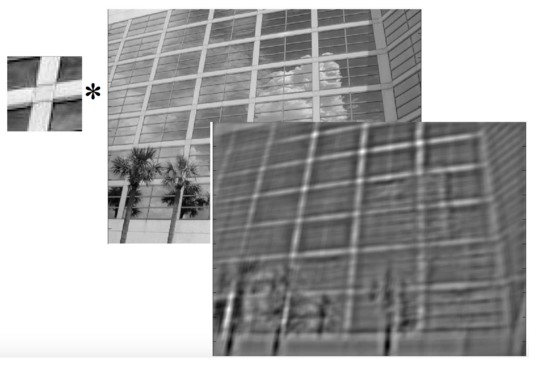 CSE/EE486 Computer Vision I, Lecture 7, Template Matching, p7
If you want to perform more strict matching, you can match not only A-> B but also B-> A and use only the ones that are judged to match on both sides. By using this feature point matching, it is possible to create panoramic photos, classify and search images.
Implementation in OpenCV
Finally, I will introduce how to implement it in OpenCV. I have a sample written in Jupyter notebook in the following repository.
icoxfog417/cv_tutorial_feature
Although it is an installation of OpenCV, Anaconda (conda) is recommended for Windows. Not only numpy and matplotlib, but also OpenCV itself can be installed in one shot from the following.
For implementation, I referred to the following OpenCV official tutorial.
The code itself is just a few lines, but it often doesn't detect well without parameter adjustments (especially SIFT), and parameter adjustments still require a theoretical understanding. In that sense, I think that a theoretical understanding is indispensable for mastering OpenCV in the true sense of the word.

We hope that the explanations introduced this time will help you to solve petrification and become a true image processing master.
Research trends
Recently, the Convolutional Neural Network (CNN) has appeared, and in terms of feature extraction from images, I think the first thing to worry about is which is better, the ancient method or CNN. First, I would like to introduce a survey on that point.
- SIFT Meets CNN: A Decade Survey of Instance Retrieval
- Object Recognition SIFT vs Convolutional Neural Networks
CNN still has some handicap in terms of learning required and processing speed, but it is still strong in that it can perform various tasks with high accuracy. Many of the ideas contained in the methods represented by SIFT are still useful, so it is proposed in the above paper that we can go higher by combining them.
Research on feature extraction using DNN includes the following.
- OverFeat: Integrated Recognition, Localization and Detection using Convolutional Networks (ICLR, 2014)
- The method that took first place in the area recognition task of ImageNet 2013. Instead of simply using CNN's Feature Map, multiple types of pooling with slightly offset (different offsets) are applied and the results are integrated. This makes it robust against misalignment. Implementation is available on GitHub
- Discriminative Learning of Deep Convolutional Feature Point Descriptors (ICCV, 2015)
- A method of inputting two image patches and learning with an error (similar or dissimilar) between them.
- You can see the GitHub implementation from the above page.
- There is also a study by the same author, "Extracting features of fashion images" (https://github.com/arXivTimes/arXivTimes/issues/255).
- Adversarial Autoencoders (2015)
- The application of GAN, which has prevailed in the generation of images, is also advancing. This is the one that uses GAN to calculate the difference between the normal distribution and the sample, which was the weak point of VAE. Click here for a summary.
- PN-Net: Conjoined Triple Deep Network for Learning Local Image Descriptors (2016)
- A method of learning with an image and a set of positive / negative images (Triple) for it, based on an idea similar to Discriminative ~.
- It seems that an improved version has been announced. This is called tfeat (BMVC, 2016), and the TensorFlow implementation is open to the public. There is also a demo of area recognition in real time.
- LIFT: Learned Invariant Feature Points (ECCV, 2016)
- Feature point detection-> (rotation) angle estimation-> (angle-independent) feature quantity description acquisition, which is the basic three processes of feature detection, realized by combining CNN.
- Adversarial Feature Learning (NIPS 2016 Workshop)
- Proposal of a Bi-directional GAN mechanism (BiGAN) that attempts to acquire the features captured by GAN by back-calculating by applying Adversarial. The use of this itself could be used in other fields as well.
- A similar study, Adversarially Learned Inference. As you can see from the Commentary site, the idea is almost the same.
References
- Practical Computer Vision To be honest, the explanation is quite blunt, and I think it is difficult for beginners to understand this alone.
- Computer Vision I
Computer Vision course at Pennsylvania State University. Very polite and easy to understand - Mobile Computer Vision
Stanford's mobile computer vision course. For a while from the introduction, we will explain how to develop Android, and from Stitching + Blending, we will explain Computer Vision. Especially recommended for those who want to embed it in mobile. - OpenCV official It's fairly straightforward and has OpenCV-based code samples. Recommended.
- Materials from the Graduate School of Information Science and Engineering, The University of Electro-Communications The story of image processing from the 9th. Rich in illustrations and easy to understand. Here is the basics of the most basic image differentiation.
- Semantic multimedia processing A2 (October 15, 2013) Click here to understand SIFT. Very easy to understand
- MIRU2013 Tutorial: SIFT and subsequent approaches Although the explanation is centered on SIFT, the systematic and historical background of the method is organized in the latter half (92-).
- VLFeat Documentation
Document of the library of feature point extraction of images that can be used in C etc. English but fairly easy to understand. - Can any one help me understand Deeply SIFT ?
- Eigenvectors, Principal Component Analysis, Covariance, Introduction to Entropy
- Image Search (Specific Object Recognition) — Classic Techniques, Matching, Deep Learning, Kaggle -gu-dian-shou-fa-matutingu-shen-ceng-xue-xi-kaggle?slide=115)
- A document that summarizes the classic methods introduced in this article to recent CNN-based methods for feature extraction from images.
Recommended Posts