[PYTHON] Speeding up numerical calculation using NumPy / SciPy: Application 1

Target

It is written for beginners of Python and NumPy. It may be especially useful for those who aim at numerical calculation of physics that corresponds to "I can use C language but recently started Python" or "I do not understand how to write like Python". Maybe.

Also, there may be incorrect statements due to my lack of study. Please forgive me.

Summary

The content is a continuation of Speeding up numerical calculation using NumPy: Basics. For loop as much as possible using universal functions and operations of ndarray. I will implement basic numerical calculation without using. SciPy will join the group from this time. I have not commented much on the detailed implementation of NumPy / SciPy functions below, so if you have any questions, please do not hesitate to contact me. Read the reference. Needless to say, ** It's very important not to reinvent the wheels. **

differential

The basic equation of physics is accompanied by the derivative. Since the derivative is a linear map, it can be described by a matrix equation. For example, let's say that we calculate the second derivative of a function. We will express this using the forward difference and the backward difference. Masu:

\frac{d^2}{dx^2}\psi(x) = \frac{\psi(x + \Delta x) - 2\psi(x) + \psi(x - \Delta x)}{\Delta x^2} + {\cal O}(\Delta x^2)

Discretize $ \ psi (x) $ with $ \ Delta x $

\psi(x)\rightarrow \{\psi(x_0), \psi(x_1), ..., \psi(x_{n-1}), \psi(x_n)\} = \{\psi_0, \psi_1, ..., \psi_{n-1}, \psi_n\}\hspace{1cm}x_i = -L/2 + i\Delta x

Derivatives can be written in matrix form:

\frac{d^2}{dx^2}\psi(x) = \frac{1}{\Delta x^2}
\begin{pmatrix}
\psi_{-1} -2\psi_0 + \psi_1\\
\psi_0 -2\psi_1 + \psi_2\\
\vdots\\
\psi_{n-2} -2\psi_{n-1} + \psi_n\\
\psi_{n-1} -2\psi_n + \psi_{n+1}
\end{pmatrix}
\simeq \frac{1}{\Delta x^2}
\begin{pmatrix}
-2&1&0&\cdots&0\\ 
1&-2 &1&&0\\
0 & 1&-2&& \vdots\\
\vdots&&&\ddots&1\\
0& \cdots& 0 &1& -2
\end{pmatrix}
\begin{pmatrix}
\psi_0\\
\psi_1\\
\vdots\\
\psi_{n-1}\\
\psi_n
\end{pmatrix}
=K\psi

There's something unpleasant about it, but it's okay if $ \ Delta x $ is small.

Implementation

I will implement it in Python. I will prepare an initial function appropriately and differentiate it:

>>> import numpy as np
>>> def f(x):
...     return np.exp(-x**2)
... 
>>> L, N = 7, 100
>>> x = np.linspace(-L/2, L/2, N)
>>> psi = f(x)
>>> psi
array([  4.78511739e-06,   7.81043424e-06,   1.26216247e-05,
         2.01935578e-05,   3.19865883e-05,   5.01626530e-05,
         7.78844169e-05,   1.19723153e-04,   1.82206228e-04,
	     ...,
         2.74540100e-04,   1.82206228e-04,   1.19723153e-04,
         7.78844169e-05,   5.01626530e-05,   3.19865883e-05,
         2.01935578e-05,   1.26216247e-05,   7.81043424e-06,
         4.78511739e-06])

And we have a matrix of derivatives. To do this we have to store the values in the inferior diagonal component. ** So we combine the slice of ndarray with np.vstack **:

>>> K = np.eye(N, N)
>>> K
array([[ 1.,  0.,  0., ...,  0.,  0.,  0.],
       [ 0.,  1.,  0., ...,  0.,  0.,  0.],
       [ 0.,  0.,  1., ...,  0.,  0.,  0.],
       ..., 
       [ 0.,  0.,  0., ...,  1.,  0.,  0.],
       [ 0.,  0.,  0., ...,  0.,  1.,  0.],
       [ 0.,  0.,  0., ...,  0.,  0.,  1.]])
>>> K_sub = np.vstack((K[1:], np.array([0] * N)))
>>> K_sub
array([[ 0.,  1.,  0., ...,  0.,  0.,  0.],
       [ 0.,  0.,  1., ...,  0.,  0.,  0.],
       [ 0.,  0.,  0., ...,  0.,  0.,  0.],
       ..., 
       [ 0.,  0.,  0., ...,  0.,  1.,  0.],
       [ 0.,  0.,  0., ...,  0.,  0.,  1.],
       [ 0.,  0.,  0., ...,  0.,  0.,  0.]])
>>> K = -2 * K + K_sub + K_sub.T
>>> K
array([[-2.,  1.,  0., ...,  0.,  0.,  0.],
       [ 1., -2.,  1., ...,  0.,  0.,  0.],
       [ 0.,  1., -2., ...,  0.,  0.,  0.],
       ..., 
       [ 0.,  0.,  0., ..., -2.,  1.,  0.],
       [ 0.,  0.,  0., ...,  1., -2.,  1.],
       [ 0.,  0.,  0., ...,  0.,  1., -2.]])

If you take the product with this, the second derivative is completed:

dx = L/N
psi_2dot = dx**-2 * np.dot(K, psi)

I could write it without using a for loop. While doing so far, ** actually there is a function to calculate the gradient called gradient **:

psi_dot_np = np.gradient(psi, dx)
psi_2dot_np = np.gradient(psi_dot_np, dx)

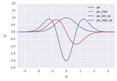
psi_2dot and psi_2dot_np almost completely overlap. You might think that the story of the matrix above doesn't make any sense, but we'll see the light of day again in the chapter on eigenvalue equations later. Will be.

Integral

A well-known algorithm for numerical integration would be Simpson's rule:

\int_a^b dx\; f(x) = \sum_{i=0}^{n-1}\frac{h}{6}\left[f(x_i) + 4f\left(x_i + \frac{h}{2}\right) + f(x_i + h)\right]\hspace{1cm}x_i = a + ih

The proof is simple with Lagrange polynomials, but I will omit it here.

Implementation

Implementing this would look like this:

>>> simp_arr = f(x) + 4 * f(x + dx / 2) + f(x + dx)
>>> dx / 6 * np.sum(simp_arr)
1.75472827313

I like the simplicity of putting the expression into the code as it is. ** However, the Simpson integral is provided as a function of SciPy: **

>>> from scipy.integrate import simps
>>> simps(psi, x)
1.7724525416390826

The calculation results are slightly different because SciPy uses the Simpson law, which is more accurate. Unless you have a specific reason, it is better to use this than to build it yourself. ** Furthermore, differentiation There is also a function that passes and integrates the previous function: **

>>> from scipy.integrate import quad
>>> quad(f, -np.inf, np.inf)
(1.7724538509055159, 1.4202636780944923e-08)

It can be calculated by giving a function and an integration interval. The return value is tuple, the first component is the integration result, and the second component is the absolute error. Quad uses the technique in the Fortran library QUADPACK. [^ 1] It seems. ** Actually, this child is very good. ** Here are some things I'm grateful for:

• ** Seems to use adaptive integrals that change the extreme width as needed **

With Simpson's rule, the width of the difference is uniform in space, but with adaptive integration, "where fine differences are needed (where the function moves violently) are fine, and where there is not much need (function movement is). It seems that it does something like "widening the width (in a calm place)". The calculation speeds up while maintaining the accuracy of the error. You may not feel so grateful with ordinary one-dimensional integration. However, when it comes to double and triple integrals, the speed is incomparable to Simpson integrals [^ 2]. It is much faster than Simpson integrals made by C / C ++.

• ** You can give np.inf to the integration interval **

For a compact function like this one, how far the integration interval is taken depends on the required calculation accuracy, but by using np.inf, the calculation accuracy is an argument of quad without worrying about the cutoff. It is good to throw it in ʻepsabs, epsrel`, etc.

• ** Easy to use **

Probably a much easier interface than touching QUADPACK directly [^ 3].

Eigenvalue equation

Now let's talk a little about quantum mechanics. Let's find the eigenfunctions and energy eigenvalues of a one-dimensional harmonic oscillator system. Hamiltonian

H = \frac{\hat{p}^2}{2} + \frac{\hat{q}^2}{2} = -\frac12\frac{d^2}{dq^2} + \frac{q^2}{2}

This is a child. It uses the unit system of $ \ hbar = \ omega = m = 1 $. Schroedinger equation for this Hamiltonian

H\psi_\ell(q) = E_\ell\psi_\ell(q)

$ \ Ell $ is not the index of the difference, but the index of the eigenvalue / eigenfunction. First, the potential term is differentiated into a matrix format:

	\frac{q^2}{2}\psi(q) \rightarrow \frac12
	\begin{pmatrix}
	q_0^2&0&0&\cdots&0\\ 
	0&q_1^2 &0&\cdots&0\\
	0 & 0&q_2^2&& \vdots\\
	\vdots&&&\ddots&0\\
	0& \cdots& 0 &0& q_n^2
	\end{pmatrix}
	\begin{pmatrix}
	\psi_0\\
	\psi_1\\
	\vdots\\
	\psi_{n-1}\\
	\psi_n
	\end{pmatrix}=\frac12
	\begin{pmatrix}
	(-L/2)^2&0&0&\cdots&0\\ 
	0&(-L/2 + \Delta q)^2 &0&&0\\
	0 & 0&(-L/2 + 2\Delta q)^2&& \vdots\\
	\vdots&&&\ddots&0\\
	0& \cdots& 0 &0& (L/2)^2
	\end{pmatrix}
	\begin{pmatrix}
	\psi_0\\
	\psi_1\\
	\vdots\\
	\psi_{n-1}\\
	\psi_n
	\end{pmatrix} = V\psi

I don't know if Hajikko will be exactly $ L / 2 $, but that's right. Recalling what we did in the derivative chapter, the Schroedinger equation is

H\psi = (K + V)\psi = \frac12
\begin{pmatrix}
\frac{2}{\Delta q^2} + (-L/2)^2&\frac{-1}{\Delta q^2}&0&\cdots&0\\ 
\frac{-1}{\Delta q^2}&\frac{2}{\Delta q^2} + (-L/2 + \Delta q)^2 &\frac{-1}{\Delta q^2}&&0\\
0 & \frac{-1}{\Delta q^2}&\frac{2}{\Delta q^2} + (-L/2 + 2\Delta q)^2&& \vdots\\
\vdots&&&\ddots&\frac{-1}{\Delta q^2}\\
0& \cdots& 0 &\frac{-1}{\Delta q^2}& \frac{2}{\Delta q^2} + (L/2)^2
\end{pmatrix}
\begin{pmatrix}
\psi_0\\
\psi_1\\
\vdots\\
\psi_{n-1}\\
\psi_n
\end{pmatrix} = E_\ell\psi

It looks like.

Implementation

Now it's coding.

#System settings
>>> L, N = 10, 200
>>> x, dx = np.linspace(-L/2, L/2, N), L / N

#Exercise term K
>>> K = np.eye(N, N)
>>> K_sub = np.vstack((K[1:], np.array([0] * N)))
>>> K = dx**-2 * (2 * K - K_sub - K_sub.T)

#Potential term
>>> V = np.diag(np.linspace(-L/2, L/2, N)**2)

#Hermitian matrix eigenvalue equation
#w is the eigenvalue,v is the eigenvector
>>> H = (K + V) / 2
>>> w, v = np.linalg.eigh(H)

The definition of dx is subtle, but don't worry:

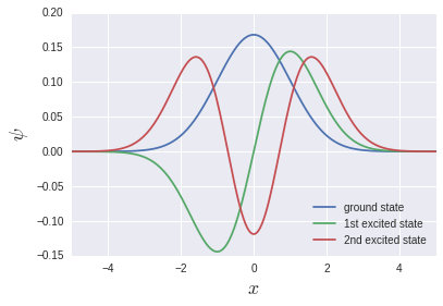
Eigenfunctions that are often seen in textbooks are output. np.linalg.eigh is a solver of eigenvalue equations for Hermitian, which returns eigenvalues and eigenfunctions. This time it is a triple diagonal matrix, so np.linalg.eig_banded for band matrices is fine. However, I think that the speed is rather faster in np.linalg.eigh [^ 4]. The memory consumption is probably less in np.linalg.eig_banded.

** It should be noted here that the ground state, the first excited state, the second excited state ... are stored in v [0], v [1], v [2] ... Instead, it means vT [0], vT [1], vT [2] .... ** This means that the storage of array data in memory is Row-major for C system and Fortran for Fortran. Probably due to the column-major discrepancy. If np.linalg.eigh is a wrapper for LAPACK, it may be a natural behavior in a sense.

Let's calculate the difference between the eigenvalues and examine the excitation energy. Let's output about 20 from the basis:

>>> np.diff(w)[:20]
[ 1.00470938  1.00439356  1.00407832  1.00376982  1.00351013  1.00351647
  1.00464172  1.00938694  1.02300462  1.05279364  1.10422331  1.17688369
  1.26494763  1.36132769  1.46086643  1.56082387  1.66005567  1.75820017
  1.85521207  1.95115074]

The excitation energy of the harmonic oscillator system is $ \ hbar \ omega $ regardless of the level, so it is 1 in this unit system. It is reproduced fairly well in the low energy region, but it becomes quite suspicious in the high energy region. Let's try to output the 15th excited state:

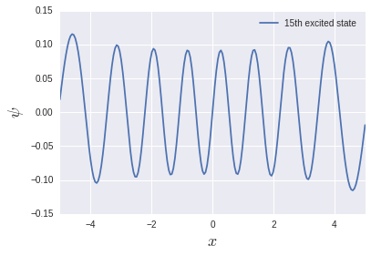
There are 15 nodes, but the function is not compact at the edges. That is why the space size of $ L = 10 $ was not enough. I want to calculate exactly which excited state. It is necessary to change the size of the space and the number of divisions.

Analytical calculation of the eigenvalues and eigenfunctions of the harmonic oscillator is a rather painstaking task, but it is very simple to throw into numerical calculations [^ 5].

Differential equation

One-dimensional diffusion equation

\frac{\partial}{\partial t}f(x, t) = \frac{\partial^2}{\partial x^2}f(x, t)

This child can find an analytical solution through the Fourier transform of $ x $ given the initial conditions [^ 6], but of course this time let's solve it by numerical calculation. Initial Give the condition in Gaussian and start with the usual spatial differentiation:

f(x, 0) = \exp(-x^2)\\
f_k \equiv f(k\Delta x, t), \hspace{0.7cm} \Delta x = L/N

Then the differential equations will also be differentiated:

\frac{d}{dt}f_0 = \frac{f_1 - 2f_0}{\Delta x^2}\\
\frac{d}{dt}f_1 = \frac{f_2 - 2f_1 + f_0}{\Delta x^2}
...\\
\frac{d}{dt}f_k = \frac{f_{k+1} - 2f_k + f_{k-1}}{\Delta x^2}\\
...\\
\frac{d}{dt}f_{n-1} = \frac{f_{n} - 2f_{n-1} + f_{n-2}}{\Delta x^2}\\
\frac{d}{dt}f_n = \frac{-2f_n + f_{n-1}}{\Delta x^2}

SciPy takes a list of differentials of a function [f0, f1, ..., fn-1, fn] as an argument and evolves it by $ \ Delta t $ over time (ndarray). There is a differential equation solver called ** ʻodeint` that can solve differential equations by passing a function that returns. **

Implementation

Let's create that function first.:

from scipy.integrate import odeint

def equation(f, t=0, N, L):
    dx = L / N
    gamma = dx**-2
    i = np.arange(1, N, 1)
    
    # f0
    arr = np.array(gamma * (f[1] - 2 * f[0]))
    # f1 to fN-1
    arr = np.append(arr, gamma * (f[i+1] - 2 * f[i] + f[i-1]))
    # fN
    arr = np.append(arr, gamma * (-2 * f[N] + f[N-1]))

    return arr

You'll somehow know what you're doing. In this function, we'll write the diffed $ f $ in the form of an array like f [n]. f isf [0] It consists of $ N + 1 $ elements fromtof [N]. Also, the first argument is a differentialized list of functions f, and the second argument is the time t. Is the specification of ʻodeint. Make sure to use this order. The initial time is of course $ t = 0 $, so the default value is set. ** # f1 to fN-1By the way, without writing[gamma * (f [j + 1] -2 * f [j] + f [j-1]) for j in i], just list ʻi which is ndarray. I think it's sober that it's OK just to put it in the index of. **

** --Addition (2016/12/3)-** After all, it's just a second derivative

from scipy.integrate import odeint

def equation(f, t=0, N, L):
    dx = L / N
    arr = np.gradient(np.gradient(f, dx), dx)

    return arr

It's good. Gradient is different from diff, and it is wonderful that the size of the list does not change after processing. -Addition here-

By the way, the initial function is

def f(x):
    return np.exp(-x**2)

It was.

Also, there are some variables that must be passed to ʻodeint itself. One is ʻequation (f, t0, ...) defined above, and the second is ndarray, which is the difference between the initial functions. (It seems to be good if iterable), the third is a list of the time t to calculate. Furthermore, ʻequation has variables other than fandt0, so their existence I have to tell odeint, so I store that information in ʻargs. Coded with these in mind:

# initial parameter(optional)
N, L = 200, 40

# coordinate
q = np.linspace(-L/2, L/2, N)
                                
# initial value for each fk
fk_0 = f(q)

# time
t_max, t_div = 10, 5
t = np.linspace(0, t_max, t_div)

trajectories = odeint(equation, fk_0, t, args=(N, L))

The time solution for t [i] is stored in trajectories [i]. Now, let's plot this:

I was able to see how Gaussian spreads. This time I dealt with the diffusion equation, so the code was a bit confusing with the two variables $ (x, t) $. The ordinary one-variable differential equation. I think it would be simpler. When plotting, we use for loops, but ... that's fine. It's important that we don't use for loops (including list inclusions) in the process of numerical calculation.

in conclusion

It's been a long time, so I'll summarize the rest in another article. If anyone says "There is a better way!", I would be grateful if you could comment.

You can see that NumPy and SciPy have a wider range of defense than I expected. When I searched for a reference thinking "Maybe ...", I already had something I had implemented myself [^ 7] That's often the case. ** It applies not only to NumPy and SciPy, but also to Python's standard modules. ** Please take a look at the Python reference. I'm sure there is a good package.

** Addendum (2016/11/25): Continued below ** Speeding up numerical calculation using NumPy / SciPy: Application 2

[^ 1]: I haven't checked if it wraps QUADPACK. The manual says "... using a technique from the Fortran library QUADPACK."

[^ 2]: I think Monte Carlo is faster than 7 or 8 layers.

[^ 3]: I haven't used it so I honestly don't know.

[^ 4]: The band matrix solver seems to calculate after expanding what passed in the band into a matrix format. Then I feel that the memory consumption does not change after all ... I do not know the details. is.

[^ 5]: Of course, physicists should not be satisfied with numerical calculations. Numerical calculations alone cannot be used for qualitative discussions, so even systems that cannot be solved exactly are approximated and analytical. It makes a lot of sense to come up with a solution.

[^ 6]: We often solve differential equations through Laplace transform in electronic circuits, but it is essentially the same. If we prepare an initial function that cannot be integrated analytically, we will end up solving it numerically. In that sense, Gaussian is a compact, analytically integrable, very good function.

[^ 7]: And often much better than what I implemented.