[PYTHON] Maximum likelihood estimation of various distributions with Pyro

Maximum likelihood estimation of various one-dimensional continuous probability distribution parameters with Pyro.

• normal distribution --Beta distribution --T distribution --Laplace distribution --Cauchy distribution --Exponential distribution --Gamma distribution --Gumbel distribution

Although maximum likelihood estimation can provide analytical solutions (normal distribution, etc.), Some are iterative (gamma distribution, etc.). In addition, the method differs depending on the distribution, and the implementation is different. Do it here using pyro, Just define the probability distribution in model After that, maximum likelihood estimation is performed by the iterative method with the same code.

Only the normal distribution will be explained in detail. Other code can be found in the gist below. https://gist.github.com/tttamaki/b061f64ad1c0f640acb2bccb88b5087e

Tips

--Use ʻAutoDeltaas a guide (point estimation) --The monitor during learning is hook --Estimates are brought in withpoutine.trace`

Preparation

Preparation. For notebook

import matplotlib.pyplot as plt
%matplotlib inline

from collections import defaultdict
import os

import numpy as np


import torch
import torch.distributions.constraints as constraints

import pyro
from pyro.optim import Adam
import pyro.distributions as dist
from pyro.infer import SVI, Trace_ELBO
from pyro.infer.autoguide import AutoDelta, AutoNormal
from pyro.infer.autoguide.initialization import init_to_feasible

# import pyro.poutine as poutine
from pyro import poutine

pyro.enable_validation(True)
pyro.set_rng_seed(101)


from tqdm.notebook import tqdm
import daft

One-dimensional normal distribution

True parameters

Randomly create true m and std

true_m = np.random.rand() * 10
true_std = np.abs(np.random.rand() * 2)
print('m =', true_m, 'std =', true_std)

x_range = np.arange(true_m - 4*true_std, true_m + 4*true_std, 0.01)
x_max = x_range.max()
x_min = x_range.min()
print('x_range: from {0:.3f} to {1:.3f}'.format(x_min, x_max))

python

m = 2.3235366181476067 std = 0.16712286732668735
x_range: from 1.655 to 2.985

Data creation

Sampling data from a true distribution

# sampling
target_dist = dist.Normal(true_m, true_std)
data = torch.tensor([target_dist() for i in range(100)])
#pdf: Distribution function
true_y = [target_dist.log_prob(torch.tensor([x])).exp() for x in x_range]


fig = plt.figure(figsize=(10,5))
plt.plot(x_range, true_y, c='k', label=r'Normal(m,$\sigma$)')
plt.hist(data, range=(x_min, x_max), bins=100, density=True, alpha=0.2, label=r'observed data $\{x_i\}$')

plt.title(r'm={0:.3f} $\sigma$={1:.3f}'.format(true_m, true_std))

plt.ylim(0,)
plt.xlabel('x')
plt.legend()
plt.savefig('obs-data')
plt.show()

By the way, the analytical solution of maximum likelihood estimation is mean and variance in the case of normal distribution.

python

ml_m = data.numpy().mean()
ml_std = data.numpy().std()
print('m={0:.3f}, sigma={1:.3f}'.format(ml_m, ml_std))

python

m=2.318, sigma=0.157

Graphical model

The model model has the following structure.

• p_\theta(X) -$ X = \ {x_1, \ ldots, x_N } $ is the observed data --Parameters are $ \ theta = \ {m, \ sigma } $
• x_i \sim \mathrm{Gauss}(m, \sigma)

Draw a graphical model with daft

pgm = daft.PGM()

pgm.add_node("xn", r"$x_n$", 2, 1, observed=True)
pgm.add_node("m", "m", 1.5, 2, fixed=True)
pgm.add_node("std", r"$\sigma$", 2.5, 2, fixed=True)
pgm.add_edge("m", "xn")
pgm.add_edge("std", "xn")
pgm.add_plate([1, 0.5, 2, 1], label=r"$n = 1, \ldots, N$", shift=-0.2)

pgm.show()  # render and show

Models and guides

For the model, set m and std as parameters in pyro.param.

model

def model(data=None):
        
    #Estimated initial value is 0.Set to 0
    m = pyro.param("m", torch.tensor(0.0))

    #Estimated initial value is 1.Set to 0
    # std >Since it is 0, add a positive constraint
    std = pyro.param("std", torch.tensor(1.0), constraint=constraints.positive)

    #data represents all the data (ie vector list array)
    with pyro.plate('observe_data'):  #Since each observation obs assumes independence, use plate
        pyro.sample('obs', dist.Normal(m, std), obs=data)  # vector-Use plate

Use point estimation AutoDelta as a guide

python

guide = AutoDelta(
    poutine.block(model, hide=['obs']),  #Hide model obs and use the others (m and std)
    init_loc_fn=init_to_feasible  #The initial value is a reasonable value
)

Estimated preparation

python

adam_params = {"lr": 0.005, "betas": (0.95, 0.999)}
optimizer = Adam(adam_params)  #Adam for the time being


svi = SVI(model=model,
          guide=guide,
          optim=optimizer,
          loss=Trace_ELBO()
         )

Parameter initialization and hook settings. To save the value in the middle of the parameter.

python

pyro.clear_param_store()  # pyro.get_param_store()Will be empty

svi.loss(model, guide, data)  #I have to do this once piro.get_param_store()Is an empty mom

trace_dic = defaultdict(list)  #Save the value (this list will be called trace here)
for name, value in pyro.get_param_store().named_parameters():
    print('tracing', name, type(value), value)
    #hook is called for each gradient calculation. Gradient value grad is ignored, name is used for param(name)Get the value with and add it to the dic list
    value.register_hook(lambda grad, name=name: trace_dic[name].append(pyro.param(name).item()))

python

tracing m <class 'torch.Tensor'> tensor(0., requires_grad=True)
tracing std <class 'torch.Tensor'> tensor(0., requires_grad=True)

Estimate

Iterative estimation.

python

num_steps = 5000

with tqdm(range(num_steps)) as pbar:
    for i,p in enumerate(pbar):

        loss = svi.step(data)  #Gradient calculation, update

        trace_dic['loss'].append(loss)

        if i > 100 and np.isclose(trace_dic['loss'][-100], loss):
            break  #Convergence if the value does not change from 100 times ago
            
        if i % 10 == 0:  #Display once every 10 times because it is too early to see
            pbar.set_postfix(loss=loss)

State of convergence

python

fig = plt.figure(figsize=(10,5))
plt.plot(trace_dic['loss'])
plt.title("ELBO")
plt.xlabel("step")
plt.ylabel("loss");
savefig("loss")
plt.show()


fig = plt.figure(figsize=(15,5))

for i,param in enumerate(['m', 'std']):
    plt.subplot(1,2,i+1)
    plt.plot(trace_dic[param])
    plt.ylabel(param)

plt.tight_layout()
savefig("params")
plt.show()

State of decrease in loss

Convergence of parameters m and std

result

Comparison of maximum likelihood estimation and true value

python

trace = poutine.trace(model).get_trace()

print('m', trace.nodes['m']['value'].item(), 'true m', true_m)
print('std', trace.nodes['std']['value'].item(), 'true std', true_std)

It is close to the true value.

python

m 5.083353042602539 true m 5.163986277024462
std 1.1655045747756958 true std 1.1413351737362796

Comparison of maximum likelihood estimation distribution and true distribution

python

fig = plt.figure(figsize=(10,5))


#Get parameters with trace
trace = poutine.trace(model).get_trace()
m = trace.nodes['m']['value'].item()
std = trace.nodes['std']['value'].item()

# generate a pdf
estimated_dist = dist.Normal(m, std)
y = [estimated_dist.log_prob(torch.tensor([x])).exp() for x in x_range]


# plot
plt.plot(x_range, y, c='k', label='ML estimated pdf')
plt.plot(x_range, true_y, c='r', label=r'true pdf')
plt.hist(data, range=(x_min, x_max), bins=100, alpha=0.2, density=True, l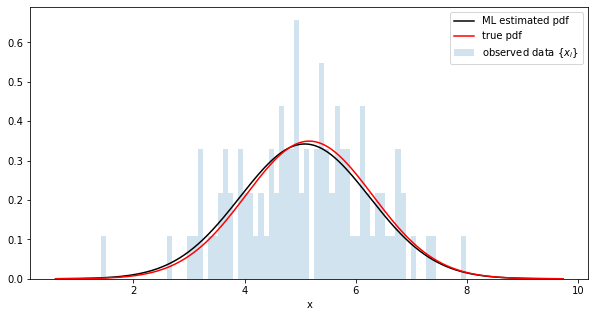![normal_sampled-pdf.png](https://qiita-image-store.s3.ap-northeast-1.amazonaws.com/0/44835/0d36d454-fce6-9b62-a42c-a8aa546733f6.png)
abel=r'observed data $\{x_i\}$')


plt.xlabel('x')
plt.legend()
savefig("sampled-pdf")
plt.show()

Sampling from the estimated distribution and comparing with the original data

python

fig = plt.figure(figsize=(10,5))

obs = []
for _ in range(5000):
    trace = poutine.trace(model).get_trace()
    obs.append(trace.nodes['obs']['value'].item())

plt.xlabel('posterior samples')

plt.hist(data, range=(x_min, x_max), bins=100, alpha=0.2, density=True, label=r'observed data $\{x_i\}$')
plt.hist(obs, range=(x_min, x_max), bins=100, alpha=0.2, density=True, color='r', label=r'sampled data$')

plt.legend()
savefig("pdf-obs")
plt.show()

Other distributions

The following shows only the original data (blue), the true distribution (red), and the estimated distribution with the maximum likelihood estimation parameters (black).

The code is https://gist.github.com/tttamaki/b061f64ad1c0f640acb2bccb88b5087e It is in.

Beta distribution

t distribution

Laplace distribution

Cauchy distribution

Exponential distribution

Gamma distribution

Gumbel distribution