[Harlem] There are too many to choose! 13 ways to calculate pi in Python
Hello from the abyss of the universe!
\displaystyle\int {\rm d}\boldsymbol{r}\hat{\psi}^{\dagger}(\boldsymbol{r})Poppin Friends\hat{\psi}(\boldsymbol{r})
is! This time, I would like to introduce ** 13 ways ** how to calculate pi $ \ pi $ in Python **!
Previously, I read an article (famous in the pi area) called "Don't worry about pi anymore! 10 ways to find π". , The desire to "seek pi" has increased, so I decided to write this article. And this time, I've implemented almost all of the methods for finding $ \ pi $ in the article ** in Python!
When I tried it, ** basic knowledge of Python ** (functions, Numpy, for statements, while statements, if statements, classes, etc.) was included ** abundantly **, so programming (like me) I highly recommend it for beginners to practice Python!
The environment is as follows.
--PC: MacBook Pro (15-inch, 2018) --CPU: 2.2 GHz 6 core Intel Core i7 --Memory: 16 GB 2400 MHz DDR4 --Python environment: Anaconda, Jupyter Notebook (6.0.1), python 3.7.4
Then, please enjoy the harem ** weaved by the methods of calculating pi!
Use the basic features of Numpy
Python has a library called Numpy (which Anaconda comes with from the beginning) and has some very useful features for vector, matrix and other math calculations. Below, we'll show you how to calculate pi with the basic features of Numpy!
- numpy.pi
The first is to use ** numpy.pi **. In Numpy, there is a guy who gives a value of pi called
numpy.pi, and it is the quickest to use this. I don't even calculate it anymore w
import numpy as np #Import numpy

pi = np.pi #Np to variable pi.Substitute pi
print(pi) #output
The output looks like this:
3.141592653589793
2. Inverse function of tan
Suppose you suddenly get hit by ** "a curse that makes only numpy.pi out of Numpy's features" **.
Now it's hard! You can't get pi with the first method! However, other features of Numpy are still available, so let's explore other ways. By the way, there is a legendary method that has been passed down since prehistoric times. It's a way to use ** tan's inverse function **.
\tan\left(\frac{\pi}{4}\right)=1\Longleftrightarrow\arctan(1)=\frac{\pi}{4}\tag{1}
If you take advantage of being
\pi = 4\arctan(1) \tag{2}
Can be asked. Let's do it!
import numpy as np

pi = 4 * np.arctan(1) #4 to variable pi*tanh(1)Substitute
print(pi) #output
The output looks like this:
3.141592653589793
I got exactly the same result as the first method! By the way, this method has been handed down from the prehistoric era when ** Fortran **, the first "language" of mankind, was born. It's the wisdom of our predecessors!
Obtained from the area
** "The area of a circle with a radius of $ r $ is $ S = \ pi r ^ 2 $" ** Speaking of, you all know that it is a universal common sense deeply engraved in the deep psychology of all humankind! Below, let's find the pi using the area of this circle that everyone knows!
3. Regular polygon approximation

By increasing the area of the regular $ n $ polygon inscribed in the circle, the value gets closer and closer to the area of the circle. The area of a regular $ n $ polygon inscribed in a circle with radius $ r $ is
S_n=n\times\frac{r^2}{2}\sin\left(\frac{360^\circ}{n}\right)\to\pi r^2\ (n\to\infty) \tag{3}
Is required at. Let's implement it assuming that the radius is $ r = 1 $!
import numpy as np

#Polygon approximation
def RegularPolygon(N):
    theta = np.radians(360 / N) #Divide 360 ° into N equal parts and convert from radian method to radian method
    pi = N * np.sin(theta) / 2 #Calculate the area of a regular N-sided polygon
    return pi

#output
print("RegularPolygon(100)     = " + str(RegularPolygon(100)))
print("RegularPolygon(1000)    = " + str(RegularPolygon(1000)))
print("RegularPolygon(10000)   = " + str(RegularPolygon(10000)))
print("RegularPolygon(100000)  = " + str(RegularPolygon(100000)))
print("RegularPolygon(1000000) = " + str(RegularPolygon(1000000)))
The function np.radius () used in the code is a function that depends on the value of pi, and it is personal to use a function that depends on pi to find the pi. It's unpleasant, but I couldn't think of any other good way, so I'm leaving it this time (please let me know if you know a good way).
The output result is as follows. It's gradually approaching pi!
RegularPolygon(100)     = 3.1395259764656687
RegularPolygon(1000)    = 3.141571982779475
RegularPolygon(10000)   = 3.141592446881286
RegularPolygon(100000)  = 3.141592651522708
RegularPolygon(1000000) = 3.1415926535691225
4. Numerical integration (rectangular approximation)
There are other ways to find the area of a circle besides polygonal approximation. This time, let's use the idea of ** integral ** (partitioned quadrature).

Consider finding the function $ y = f (x) $, the straight line $ x = a, \ x = b \ (a <b) $, and the area $ S $ of the part enclosed by the $ x $ axis. $ x $ Axis interval $ [a, \ b] $ is divided into $ n $ equal parts, and the equal division points are $ x_0, \ x_1, \ x_2, \ cdots, \ x_n \ (where \ x_0 = a, \ Let x_n = b) $. Also, let the interval between adjacent equinoxes be $ \ Delta x = (b-a) / n $. At this time, the area $ S_i $ of the interval $ [x_i, \ x_ {i + 1}] $ is ** $ S_i = f (x_i) \ Delta x $ **, that is, the base is $ \ Delta x. Approximate as a rectangle with $ and height of $ f (x_i) $ **. After that, find $ S_i $ for all intervals $ [x_i, \ x_ {i + 1}] \ (i = 0, \ 2, \ cdots, \ n-1) $, and add them up to approximate. Area $ S_n $ can be obtained. Then, if you increase the number $ n $ that divides the interval $ [a, \ b] $ into equal parts, it will eventually approach the true area $ S $.
S_n = \sum_{i=0}^{n-1} f(x_i)\frac{b-a}{n}\to S\ (n\to\infty) \tag{4}
Let's apply this method to the area of a circle. The equation for the unit circle (center of origin, radius 1) in the $ x-y $ plane is
x^2+y^2=1\Longleftrightarrow y=\pm\sqrt{1-x^2} \tag{5}
However, the plus one represents the upper half and the minus one represents the lower half. This time, find the area of the part (quarter circle) of $ x> = 0 $ in the upper half. The interval of the area to be calculated is $ [a, \ b] = [0, \ 1] $, so if this is applied to the formula (4) of the division quadrature
S_n=\sum_{i=0}^{n-1} \frac{\sqrt{1-\left(\frac{i}{n}\right)^2}}{n}\to \frac{\pi}{4}\ (n\to\infty) \tag{6}
It will be.
Let's implement it!
import numpy as np

#Rectangle approximation function. section[0,1]Is divided into N equal parts.
def Rectangle(N):
    x = np.arange(N) / N #0~(N-1)/N element array up to N
    y = np.sqrt(1 - x**2) #y=root(1-x^2)Calculate
    pi = 4 * np.sum(y) / N #Calculate area
    return pi

#output
print("Rectangle(100)     = " + str(Rectangle(100)))
print("Rectangle(1000)    = " + str(Rectangle(1000)))
print("Rectangle(10000)   = " + str(Rectangle(10000)))
print("Rectangle(100000)  = " + str(Rectangle(100000)))
print("Rectangle(1000000) = " + str(Rectangle(1000000)))
The result is as follows
Rectangle(100)     = 3.160417031779046
Rectangle(1000)    = 3.1435554669110277
Rectangle(10000)   = 3.141791477611322
Rectangle(100000)  = 3.1416126164019866
Rectangle(1000000) = 3.141594652413813
Convergence is slower than the polygon approximation, but the value converges to pi as the even fraction $ n $ increases.
5. Numerical integration (trapezoidal approximation)
Just by adding ** a twist to the previous division quadrature, the accuracy will be considerably higher than the rectangular approximation **. Earlier, the area of the minute section was approximated by a rectangle, but it is ** upper base $ f (x_i) $, lower base $ f (x_ {i + 1}) $, height $ \ Delta x $ Approximate as a trapezoid **. In other words, use the following formula.
S_n = \sum_{i=0}^{n-1} \frac{f(x_i)+f(x_{i+1})}{2}\cdot\frac{b-a}{n}\to S\ (n\to\infty) \tag{7}
As you can see in the figure below, the rectangle approximation has a lot of extra or missing parts at the top, but the trapezoidal shape reduces it considerably.

Let's implement it!
import numpy as np

#Trapezoidal approximation
def Trapezoid(N):
    x = np.arange(N + 1) / N #0~N + 1 element array up to 1
    y = np.sqrt(1 - x**2) #y=root(1-x^2)Calculate
    z = (y[0:N] + y[1:N+1]) / 2 #Trapezoidal(Upper base + lower base)/Calculate 2
    pi = 4 * np.sum(z) / N #Calculate area
    return pi

#output
print("Trapezoid(100)     = " + str(Trapezoid(100)))
print("Trapezoid(1000)    = " + str(Trapezoid(1000)))
print("Trapezoid(10000)   = " + str(Trapezoid(10000)))
print("Trapezoid(100000)  = " + str(Trapezoid(100000)))
print("Trapezoid(1000000) = " + str(Trapezoid(1000000)))
The following is the execution result. It is slightly inferior to the polygon approximation, but it can be seen that the convergence is faster than the rectangle approximation.
Trapezoid(100)     = 3.1404170317790454
Trapezoid(1000)    = 3.141555466911028
Trapezoid(10000)   = 3.141591477611322
Trapezoid(100000)  = 3.1415926164019865
Trapezoid(1000000) = 3.1415926524138094
Find from the series
There is a way to express pi using an infinite series, which is the sum of an infinite sequence of numbers. Let's use it to find the pi! (In addition, the proof is quite troublesome or impossible for the author, so I will omit it ...)
6. Basel series
It is known that pi appears in the following series.
1+\frac{1}{2^2}+\frac{1}{3^2}+\dots+\frac{1}{n^2}+\dots=\sum_{n=1}^\infty\frac{1}{n^2}=\frac{\pi^2}{6} \tag{8}
The formula is the sum of all the reciprocals of the squares of natural numbers, but surprisingly, the result includes pi. When I'm doing math, it's interesting to enjoy the fun of "Does $ \ pi $ come out there!" Click here for details on Basel series
As in the case of numerical integration, it is impossible for a computer to perform operations that continue indefinitely, so here we cut off the sum in the middle and find an approximate value. Let's implement it!
import numpy as np

#Basel series. Calculate the sum up to the Nth term.
def Basel(N):
    x = np.arange(1, N + 1) #1~Array of natural numbers up to N
    pi = np.sqrt(6 * np.sum(1 / x**2)) #Calculate the inverse sum of squares for each element of the array and multiply by 6 to square.
    return pi

#output
print("Basel(100)     = " + str(Basel(100)))
print("Basel(1000)    = " + str(Basel(1000)))
print("Basel(10000)   = " + str(Basel(10000)))
print("Basel(100000)  = " + str(Basel(100000)))
print("Basel(1000000) = " + str(Basel(1000000)))
Below are the results. You can see that as the number of terms to be summed increases, it converges to pi.
Basel(100)     = 3.132076531809106
Basel(1000)    = 3.1406380562059932
Basel(10000)   = 3.14149716394721
Basel(100000)  = 3.1415831043264415
Basel(1000000) = 3.1415916986604673
7. Leibniz series
There are other series that give pi. The Leibniz series below is one of them.
1-\frac{1}{3}+\frac{1}{5}-\frac{1}{7}+\dots+\frac{(-1)^{n-1}}{2n-1}+\dots=\sum_{n=1}^\infty\frac{(-1)^{n-1}}{2n-1}=\frac{\pi}{4} \tag{9}
This time, the calculation is to add the reciprocals of odd numbers alternately plus and minus, but the pi appears here as well! Click here for details on Leibniz series
Let's implement it in the same way as the Basel series.
import numpy as np

#Leibniz series. Calculate the sum up to the Nth term.
def Leibniz(N):
    x = np.arange(1, N + 1) #1~Array of natural numbers up to N
    y = 1 / (2 * x - 1) #Compute an array of odd reciprocals
    pm = (-1) ** (x - 1) #Calculation of a sequence of alternating Pramai 1
    pi = 4 * np.dot(y, pm) #Calculate the sum of alternating Pramai by the inner product of y and pm, and multiply by 4 at the end.
    return pi

#output
print("Leibniz(100)     = " + str(Leibniz(100)))
print("Leibniz(1000)    = " + str(Leibniz(1000)))
print("Leibniz(10000)   = " + str(Leibniz(10000)))
print("Leibniz(100000)  = " + str(Leibniz(100000)))
print("Leibniz(1000000) = " + str(Leibniz(1000000)))
The following is the execution result. It's converging smoothly!
Leibniz(100)     = 3.131592903558553
Leibniz(1000)    = 3.140592653839795
Leibniz(10000)   = 3.141492653590045
Leibniz(100000)  = 3.141582653589825
Leibniz(1000000) = 3.141591653589752
8. Ramanujan series
Finally, I would like to introduce the monster-like series ** "Ramanujan series" **. The following is the formula.
\begin{align}
\frac{1}{\pi} = \frac{2\sqrt{2}}{99^2}\sum_{n=0}^\infty\frac{(4n)!(1103+26390n)}{(396^{n}n!)^4} \tag{10}
\\
\frac{4}{\pi} = \sum_{n=0}^\infty\frac{(-1)^n(4n)!(1123+21460n)}{882^{2n+1}(4^n n!)^4} \tag{11}
\end{align}
I don't understand the meaning anymore. .. .. Ramanujan is an Indian mathematician who has left behind a number of incomprehensible formulas such as the ones above. Also, when asked "How did you come up with the ceremony," he answered, "The goddess will teach you in your dreams." It's a metamorphosis. Click here for details on Ramanujan series [Click here for Ramanujan](https://ja.wikipedia.org/wiki/%E3%82%B7%E3%83%A5%E3%83%AA%E3%83%8B%E3%83%B4% E3% 82% A1% E3% 83% BC% E3% 82% B5% E3% 83% BB% E3% 83% A9% E3% 83% 9E% E3% 83% 8C% E3% 82% B8% E3% 83% A3% E3% 83% B3)
Let's implement it! This time, I will implement equation (11) in my mood.
import numpy as np

#Ramanujan series. Sum up to the Nth term.
def Ramanujan(N):
    sum = 0.0 #The value of the sum. Initial value 0
    for i in range(N): #i is 0 to N-Do less than 1
        numerator = ((-1)**i) * np.math.factorial(4 * i) * (1123 + 21460 * i) #Calculation of numerator of term i
        denominator = (882**(2 * i + 1)) * ((4**i) * np.math.factorial(i))**4 #Calculation of the denominator of paragraph i
        sum = sum + numerator / denominator #Add term i to sum
    pi = 4 / sum #Calculation of pi
    return pi

#output
print("Ramanujan(1) = " + str(Ramanujan(1)))
print("Ramanujan(2) = " + str(Ramanujan(2)))
print("Ramanujan(3) = " + str(Ramanujan(3)))
print("Ramanujan(4) = " + str(Ramanujan(4)))
print("Ramanujan(5) = " + str(Ramanujan(5)))
Since the Ramanujan series converges very quickly, and the factorial ($ n! $) Appearing in the formula has a rapid divergence and may overflow if a large value is entered, the term to be summed is the Basel series or Much less than the Leibniz series.
Below are the results. Even the first item matches up to the fourth decimal place, and the third and subsequent items have the same value within the range of the number of digits displayed on the personal computer. It's an overwhelming speed of convergence!
Ramanujan(1) = 3.1415850400712375
Ramanujan(2) = 3.141592653597622
Ramanujan(3) = 3.1415926535897936
Ramanujan(4) = 3.1415926535897936
Ramanujan(5) = 3.1415926535897936
Use random numbers
You can also find $ \ pi $ by using random numbers. Random numbers, as the name implies, are random numbers, such as the roll of a dice. However, finding $ \ pi $ using random numbers requires a large number of samples ($ \ sim $ millions), and it is too boring for humans to roll a million dice. The troublesome routine work is to introduce a computer to improve efficiency, so below we will introduce how to find $ \ pi $ using random numbers!
9. Monte Carlo method

Consider a $ 1 \ times 1 $ square and a quadrant centered on one of its vertices. The area ratio of the square to the quadrant is $ 1: \ pi / 4 $. Dots will be made completely randomly within this square. When the number of points increases, it becomes "total number of points: number of points contained inside the quadrant $ \ simeq1: \ pi / 4 $". For example, if $ n $ of $ N $ points are included in the quadrant,
\frac{n}{N}\simeq\frac{\pi}{4} \tag{12}
It will be. Use this to find the pi.
Let's implement it!
import numpy as np

#Monte Carlo method. Take N samples.
def MonteCarlo(N):
    xy = np.random.rand(2, N) #section[0,1)Uniformly distributed random numbers(2×N)queue. Each column corresponds to the coordinates of a point on the plane.
    r = np.sum(xy**2, axis = 0) #Calculate the distance from the origin of each sample point. Square each component and sum the elements in the same column.
    r = r[r<=1] #Distance is 1 or less (=Extract only samples (inside the quadrant)

    n = r.size #Calculate the number of points in the circle#Calculate pi

    pi = 4 * n / N #Calculate pi
    return pi

np.random.seed(seed=0) #Random number seed setting (doing this will result in the same output each time)

#output
print("MonteCarlo(100)       = " + str(MonteCarlo(100)))
print("MonteCarlo(1000)      = " + str(MonteCarlo(1000)))
print("MonteCarlo(10000)     = " + str(MonteCarlo(10000)))
print("MonteCarlo(100000)    = " + str(MonteCarlo(100000)))
print("MonteCarlo(1000000)   = " + str(MonteCarlo(1000000)))
print("MonteCarlo(10000000)  = " + str(MonteCarlo(10000000)))
Below are the results. In general, the error of the value due to random numbers converges on the order of $ 1 / \ sqrt {N} $ for the number of samples $ N $ (relatively slow), so the accuracy is quite low.
MonteCarlo(100)       = 3.24
MonteCarlo(1000)      = 3.068
MonteCarlo(10000)     = 3.1508
MonteCarlo(100000)    = 3.13576
MonteCarlo(1000000)   = 3.140048
MonteCarlo(10000000)  = 3.1424264
10. Buffon's needle

Drop a lot of $ l $ length needles on a lot of parallel lines drawn at intervals of $ t $. Let $ n $ be the number of $ N $ needles that intersect the line. When the number of needles $ N $ is large enough
\frac{2lN}{tn}\sim\pi \tag{13}
Is known to be. You've come again, it's the one who says "Does $ \ pi $ come out here!" W It's a seemingly strange thing that the probability of pi appears even though you just drop the needle on the parallel line. happen. Click here for details on Buffon's needle
Let's implement it! The distance between the center of the needle and the line is uniform at $ 0 \ sim t / 2 $, and the angle between the needle and the parallel line is uniform at $ 0 ^ \ circ \ sim 90 ^ \ circ $. Also, this time, the needle length is $ l = 2 $ and the parallel line spacing is $ t = 4 $.
There are some things to be careful about when sampling the needle angle from random numbers. It is necessary to convert the radius method to the radian method when directly sampling the angle, but the np.radius () that will be used in this case is a function that depends on the value of pi. .. Simulation can be done using it, but I personally feel uncomfortable, so I will devise a little this time. ** Sample the coordinates of a point in a unit quadrant and find the value of sin from it **. By limiting the range of sample points to the unit quadrant, the angle between the point and the $ x $ axis can be reduced.
It has a uniform distribution of $ 0 ^ \ circ \ sim 90 ^ \ circ $.
import numpy as np

#Buffon's needle. Drop N needles.
def Buffon(N):
    n = 0; #The number of needles that overlap the line. Initial value 0.
    for i in range(N): #i is 0 to N-Repeat until 1.
        #Needle angle sampling. Eliminate the value dependency of pi by sampling points within the unit circle instead of directly sampling the angle.
        r = 2 #Distance from the origin of the sample point. Set the initial value to 2 to execute the following while statement.
        while r > 1: #r<=Repeat the sample until it reaches 1.
            dx = np.random.rand() #x coordinate
            dy = np.random.rand() #y coordinate
            r = np.sqrt(dx ** 2 + dy ** 2) #Calculation of distance from origin

        h = 2 * np.random.rand() + dy / r #Calculation of the height (higher) of the tip of the tuft
        if h > 2: #When the height of the tip of the needle finishes the height of the parallel line
            n += 1 #Add the number of needles that overlap the line

    pi = N / n #Calculation of pi
    return pi

np.random.seed(seed=0) #Random number seed setting (doing this will result in the same output each time)

#output
print("Buffon(100)        = " + str(Buffon(100)))
print("Buffon(1000)       = " + str(Buffon(1000)))
print("Buffon(10000)      = " + str(Buffon(10000)))
print("Buffon(100000)     = " + str(Buffon(100000)))
print("Buffon(1000000)    = " + str(Buffon(1000000)))
print("Buffon(10000000)   = " + str(Buffon(10000000)))
Generate the angle of $ N $ needles with theta = np.radians (rand.rand (N) * 90). Since rand.rand () has a uniform distribution of the interval $ [0, 1) $, multiplying it by 90 gives a uniform distribution of $ [0, 90) $.
Then calculate the $ y $ coordinates of the needle tip with y = 2 * rand.rand (N) + np.sin (theta). 2 * rand.rand (N) is used to calculate the coordinates of the center of the needle, and np.sin (theta) is used to calculate the difference in height between the center and tip of the needle. Whether or not the tip of the needle intersects the parallel line is determined by [y> 2](if $ y> 2 $, it intersects, otherwise it does not intersect). After that, calculate the number of needles that intersect with y.size, and if you mess up, you're done.
The following is the output result. The result is not stable. .. .. (Sweat)
Buffon(100)        = 2.7777777777777777
Buffon(1000)       = 2.881844380403458
Buffon(10000)      = 3.1259768677711786
Buffon(100000)     = 3.11284046692607
Buffon(1000000)    = 3.1381705093564554
Buffon(10000000)   = 3.1422055392056127
Use an algorithm
A ** algorithm ** is, roughly speaking, a ** summary of a particular procedure **. Below, we'll show you how to find pi by repeating certain steps!
11. Gauss-Legendre's algorithm
The Gauss-Legendre algorithm is a method of calculating pi according to the procedure of "repeating the terms of a sequence according to a simultaneous recurrence formula" as follows.
\begin{align}
&a_0=1,\quad b_0=\frac{1}{\sqrt{2}},\quad t_0=\frac{1}{4},\quad p_0=1\\
&a_{n+1}=\frac{a_n+b_n}{2}\\
&b_{n+1}=\sqrt{a_nb_n}\\
&t_{n+1}=t_n-p_n(a_n-a_{n+1})^2\\
&p_{n+1}=2p_n\\
\\
&\frac{a_n+b_n}{4t_n}\to\pi(n\to\infty)
\end{align}
\tag{14}
This algorithm is known to approximately double the number of digits that match the exact value as the calculation progresses, making it easy and accurate to determine pi. Gauss and Legendre, who independently devised this algorithm, are both superstars in the mathematical and physics world. Click here for details on the Gauss-Legendre algorithm [Click here for details on Gauss](https://ja.wikipedia.org/wiki/%E3%82%AB%E3%83%BC%E3%83%AB%E3%83%BB%E3%83%95 % E3% 83% AA% E3% 83% BC% E3% 83% 89% E3% 83% AA% E3% 83% 92% E3% 83% BB% E3% 82% AC% E3% 82% A6% E3 % 82% B9) [Click here for details on Legendre](https://ja.wikipedia.org/wiki/%E3%82%A2%E3%83%89%E3%83%AA%E3%82%A2%E3%83%B3 % EF% BC% 9D% E3% 83% 9E% E3% 83% AA% E3% 83% BB% E3% 83% AB% E3% 82% B8% E3% 83% A3% E3% 83% B3% E3 % 83% 89% E3% 83% AB)
Let's implement it!
import numpy as np

#Gauss=Legendre's algorithm. Repeat N times
def GaussRegendre(N):
    #First term
    a = 1.0
    b = np.sqrt(2) / 2
    t = 1 / 4
    p = 1

    for i in range(N): #i is 0 to N-Repeat the following until 1
        #Calculate the following terms according to the recurrence formula
        a_new = (a + b) / 2
        b_new = np.sqrt(a * b)
        t_new = t - p * (a - a_new)**2
        p_new = 2 * p

        #Replace old value with new value
        a = a_new
        b = b_new
        t = t_new
        p = p_new

    pi = (a + b)**2 / (4 * t) #Calculation of pi
    return pi

#output
print("GaussRegendre(1) = " + str(GaussRegendre(1)))
print("GaussRegendre(2) = " + str(GaussRegendre(2)))
print("GaussRegendre(3) = " + str(GaussRegendre(3)))
Below are the results. The first time is up to the second decimal place, the second time is up to the seventh decimal place, and the third time is up to the last digit displayed. Convergence is pretty fast!
GaussRegendre(1) = 3.1405792505221686
GaussRegendre(2) = 3.141592646213543
GaussRegendre(3) = 3.141592653589794
Use physics
Pi is hidden not only in the world of mathematics but also in the natural world. Below, we'll show you how to use physics to calculate pi!
12. Simple vibration cycle
In physics, motions such as ** vibration ** have been actively studied, but simple vibration is the basis of all periodic motions. Simple vibration is the motion when the position $ x $ follows the following equation.
\frac{d^2x}{dt^2}=-\omega^2x \tag{15}
An equation that includes the differential of a function, such as equation (15), is called a ** differential equation **. Many differential equations in the world cannot be solved exactly, but equation (15) can be solved exactly, and the solution is as follows.
x=A\sin(\omega t + \phi) \tag{16}
You can see that $ x $ oscillates over time because the position $ x $ is represented by $ \ sin $ as a function of time $ t $. $ A $ is the amplitude of the vibration and $ \ phi $ is a constant called the initial phase, which is related to the position of the object at $ t = 0 $. And the period of this vibration is
T=\frac{2\pi}{\omega} \tag{17}
It will be. If $ \ omega = 1 $, the half cycle of vibration is the pi.
This time, we will calculate the vibration period by numerically simulating the differential equation. The ** Runge-Kutta method ** is used to simulate the differential equations. Since the detailed explanation of the Runge-Kutta method is long, I will omit it here, but briefly, "Find the position and velocity value in the future from the position and velocity value at a certain time according to a certain procedure. It is a way to repeat that.
\begin{align}
&Time interval:h,\quad differential equation:\frac{dx}{dt}=f(x, t)\\
&{k}_1=h\times {f}(x_i, t)\\
&{k}_2=h\times {f}(x_i+\frac{k_1}{2}, t+\frac{h}{2})\\
&{k}_3=h\times {f}(x_i+\frac{k_2}{2}, t+\frac{h}{2})\\
&{k}_4=h\times {f}(x_i+k_3, t+h)\\
\\
&{k}=\frac{{k}_1+2{k}_2+2{k}_3+{k}_4}{6}\\
&x_{i+1}=x_i+{k}
\end{align}
\tag{18}
Click here for a detailed explanation of the Runge-Kutta method
I have written another article using the Runge-Kutta method, so please read it if you like! Simulation of chaos in Unity using Runge-Kutta method
Let's implement it! The Runge-Kutta method of Eq. (18) is used for the first-order differential equation by default, but since the differential equation of Eq. (15) is the second-order differential equation, it is divided into two first-order differential equations as follows. I will end up.
\begin{align}
&\frac{dx}{dt}=v\\
&\frac{dv}{dt}=-\omega^2x
\end{align}
\tag{19}
The initial position and initial velocity are $ (x_0, v_0) = (1,0) $. In this way, the motion of the object starts from the highest point of vibration. After that, the position decreases for a while, reaches the lowest point of vibration just after half a cycle, and then the position rises. Then, by advancing the time only while the position of the object is decreasing and censoring it when the position is increasing, a half-cycle time (≈pi) can be obtained.

import numpy as np

#Differential equation. r:Vector summarizing position and velocity
def f(r):
    x = r[0] #Take out the value of the position
    v = r[1] #Get the speed value

    #Calculate the right side of the differential equation
    xdot = v
    vdot = -x

    return np.array([xdot, vdot])

#Runge=Kutta method
def RungeKutta(r, h):
    k1 = h * f(r)
    k2 = h * f(r + k1 / 2)
    k3 = h * f(r + k2 / 2)
    k4 = h * f(r + k3)

    k = (k1 + 2 * k2 + 2 * k3 + k4) / 6

    return r + k

#Simple vibration. Time interval h=10^(-N)Perform the Runge-Kutta method.
def Vibration(N):
    h = 10**(-N) #calculation of h
    t = 0 #Initial value of an integer corresponding to the time
    isDecrease = True #Flag of whether the position is decreasing
    r = np.array([1.0, 0.0]) #Initial value of position / velocity
    x_old = r[0] #Initial value substitution at the old position. Used to judge the increase / decrease of the position.

    while isDecrease == True and t * h < 4.0: #Repeat the following while the position decreases and the time is 4 or less.
    #※t*h<4.Imposing 0 prevents you from entering an infinite loop

        r = RungeKutta(r, h) #Runge=Update position and speed with Kutta method
        x_new = r[0] #New position value

        if x_old > x_new: #The old position is larger than the new position (=If the position is decreasing)
            x_old = x_new #Replace the old position value
            t += 1 #Advance the time
        else : #Otherwise
            isDecrease = False #Flag that is decreasing to False → Loop ends
    pi = t / 10 ** N
    return pi #Half cycle(≒π)return it

#output
print("Vibration(1) = " + str(Vibration(1)))
print("Vibration(2) = " + str(Vibration(2)))
print("Vibration(3) = " + str(Vibration(3)))
print("Vibration(4) = " + str(Vibration(4)))
print("Vibration(5) = " + str(Vibration(5)))
Below are the results. You can see that the smaller the width of $ h $, the higher the accuracy. However, it will take time because the number of loops required will increase accordingly.
Vibration(1) = 3.1
Vibration(2) = 3.14
Vibration(3) = 3.142
Vibration(4) = 3.1416
Vibration(5) = 3.14159
13. Number of collisions between two balls
As the thirteenth, that is, the last method, I will introduce the impact method for finding the pi. It is said that ** the number of collisions between two balls and a wall is the pi **. I don't know what you're talking about, so I'll post a video and the original paper.
Video: 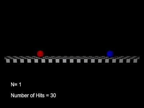
Original paper: PLAYING POOL WITH π (THE NUMBER π FROM A BILLIARD POINT OF VIEW)
Prepare two balls with a mass ratio of $ 1: 100 ^ N $, and hit the light ball at a speed of 1 while keeping the light ball stationary. Prepare a wall ahead of the light ball after the collision so that it bounces off with a coefficient of restitution of 1. After repeated collisions, the heavy ball will move in the opposite direction of the wall, and the light ball will not collide when it cannot catch up with the heavy ball. If you count the number of times a light ball collides with a heavy ball and a wall so far, it will be the number of $ N $ digits of pi.
Let's implement it! First, calculate the change in velocity due to collision in advance. The calculation method is a combination of the ** law of conservation of momentum ** and the ** definition formula of the coefficient of restitution **, which are familiar in high school physics. Let the velocities of the light and heavy spheres before the collision be $ v and V $, respectively, and the velocities after the collision be $ v'and V'$, respectively. Let the mass ratio of the light sphere and the heavy sphere be $ 1: r $. At this time, the following two equations hold before and after the collision.
\begin{align}
&v+rV=v'+rV'\\
&e=-\frac{v'-V'}{v-V}
\end{align}
\tag{20}
This time, all collisions are elastic collisions, so $ e = 1 $. Solving the simultaneous equations for $ v', V'$
v'=\frac{(1-r)v+2rV}{1+r},\quad V'=\frac{2v+(r-1)V}{1+r} \tag{21}
It will be. Based on this, let's implement it!
#Two-ball collision. Find up to the Nth digit.
def BallCollision(N):
    v = 0.0  #Initial velocity of light ball
    V = -1.0 #Initial velocity of heavy ball
    r = 100 ** N #Mass ratio
    count = 0 #Initial value of the number of collisions

    while v > V: #Repeat the following while the velocity of the light ball is greater than the velocity of the heavy ball
        v_new = ((1 - r) * v + 2 * r * V) / (r + 1) #Velocity of light ball after collision
        V_new = (2 * v + (r - 1) * V) / (r + 1) #Velocity of heavy ball after collision
        count += 1 #Added number of collisions

        if(v_new < 0.0): #When the speed of the light ball is negative
            v_new = -v_new #Speed reverses due to collision with wall
            count += 1 #Added number of collisions

        v = v_new #Replacing the speed of a light ball
        V = V_new #Heavy ball velocity replacement

    pi = count / (10 ** N) #Calculation of pi
    return pi

#output
for i in range(8):
    print("BallCollision(" + str(i) + ") = " + str(BallCollision(i)))
The following is the execution result. You really want the pi to the Nth digit! However, the amount of calculation increases 100 times to increase the accuracy by one digit, so it seems to be inconvenient.
BallCollision(0) = 3.0
BallCollision(1) = 3.1
BallCollision(2) = 3.14
BallCollision(3) = 3.141
BallCollision(4) = 3.1415
BallCollision(5) = 3.14159
BallCollision(6) = 3.141592
BallCollision(7) = 3.1415926
I tried to put it all together in the class
Finally, I've put together a class of all the techniques I've implemented so far! If you collect all of them in this way, it's quite a volume. .. .. !!
#Class Pi_Description of Harem
#A harem class woven by 13 methods for finding pi.
#Find the pi the way you like!
#* Import numpy as np is required to use.
#
#Function description:
#All functions have a return value.
#    1.  pi() :
#        np.Returns the value of pi. No arguments.
#
#     2.  Arctan() :
#        4*np.arctan(1)Returns the value of. No arguments.
#
#    3.  RegularPokygon(N) :
#Find the pi from the area of a regular polygon and return the value. Argument N = number of vertices in the regular polygon.
#
#    4.  Rectangle(N) :
#Find the pi from the numerical integration (rectangular approximation) and return the value. Argument N = equal fraction of the integration interval.
#
#    5.  Trapezoid(N) :
#Find the pi from numerical integration (trapezoidal approximation) and return the value. Argument N = equal fraction of the integration interval.
#
#    6.  Basel(N) :
#Find the pi from the Basel series and return the value. Argument N = number of terms that take the sum.
#
#    7.  Leibniz(N) :
#Find the pi from the Leibniz series and return the value. Argument N = number of terms that take the sum.
#
#    8.  Ramanujan(N) :
#Find the pi from the Ramanujan series and return the value. Argument N = number of terms that take the sum.
#
#    9.  MonteCarlo(N) :
#Find the pi from the Monte Carlo quadrature of the quadrant and return the value. Argument N = number of samples.
#
#    10. Buffon(N) :
#Find the pi from Buffon's needle simulation and return the value. Argument N = number of samples.
#
#    11. GaussRegendre(N) :
#Gauss=Find the pi from the Legendre algorithm and return the value. Argument N = number of algorithm iterations.
#
#    12. Vibration(N) :
#Obtain the pi from the simulation of simple vibration and return the value. Argument N = Variable that determines the step width h of time. h=10^(-N)
#
#    13. BallCollision(N) :
#Find the pi from the simulation of the collision of two balls and return the value. Argument N = number of digits you want to find.

import numpy as np

#Class definition
class Pi_Harem():
    #Basic features of Numpy
    # 1.Exact value of π(numpy.Use pi)
    def pi(self):
        return np.pi

    # 2.Inverse function of tan
    def Arctan(self):
        return 4 * np.arctan(1)

    #area
    # 3.Polygon approximation
    def RegularPolygon(self, N):
        theta = np.radians(360 / N)
        pi = N * np.sin(theta) / 2

        return pi

    # 4.Rectangle approximation
    def Rectangle(self, N):
        x = np.arange(N) / N
        y = np.sqrt(1 - x**2)
        pi = 4 * np.sum(y) / N

        return pi

    # 5.Trapezoidal approximation
    def Trapezoid(self, N):
        x = np.arange(N + 1) / N
        y = np.sqrt(1 - x**2)
        z = (y[0:N] + y[1:N+1]) / 2
        pi = 4 * np.sum(z) / N

        return pi

    #series
    # 6.Basel series
    def Basel(self, N):
        x = np.arange(1, N + 1)
        pi = np.sqrt(6 * np.sum(1 / x**2))

        return pi

    # 7.Leibniz series
    def Leibniz(self, N):
        x = np.arange(1, N + 1)
        y = 2 * x - 1
        pi = 4 * np.dot(1 / y, (-1)**(x - 1))

        return pi

    # 8.Ramanujan series
    def Ramanujan(self, N):
        sum = 0.0

        for i in range(N):
            numerator = ((-1)**i) * np.math.factorial(4 * i) * (1123 + 21460 * i)
            denominator = (882**(2 * i + 1)) * ((4**i) * np.math.factorial(i))**4
            sum = sum + np.sum(numerator / denominator)

        pi = 4 / sum

        return pi

    #random number
    # 9.Monte Carlo method
    def MonteCarlo(self, N):
        xy = np.random.rand(2, N)
        r = np.sum(xy**2, axis = 0)
        r = r[r<=1]
        n = r.size

        pi = 4 * n / N

        return pi

    # 10.Buffon's needle
    def Buffon(self, N):
        n = 0;
        for i in range(N):
            r = 2
            while r > 1:
                dx = np.random.rand()
                dy = np.random.rand()
                r = np.sqrt(dx ** 2 + dy ** 2)

            h = 2 * np.random.rand() + dy / r
            if h > 2:
                n += 1

        pi = N / n
        return pi

    #algorithm
    # 11.Gauss=Legendre's algorithm
    def GaussRegendre(self, N):
        a = 1.0
        b = np.sqrt(2) / 2
        t = 1 / 4
        p = 1

        for i in range(N):
            a_new = (a + b) / 2
            b_new = np.sqrt(a * b)
            t_new = t - p * (a - a_new)**2
            p_new = 2 * p

            a = a_new
            b = b_new
            t = t_new
            p = p_new

        pi = (a + b)**2 / (4 * t)
        return(pi)

    #Physics
    # 12.Simple vibration
    #Differential equation(Private function)
    def __f(self, r):
        x = r[0]
        v = r[1]
        xdot = v
        vdot = -x
        return np.array([xdot, vdot])

    #Runge-Kutta method(Private function)
    def __RungeKutta(self, r, h):
        k1 = h * self.__f(r)
        k2 = h * self.__f(r + k1 / 2)
        k3 = h * self.__f(r + k2 / 2)
        k4 = h * self.__f(r + k3)

        k = (k1 + 2 * k2 + 2 * k3 + k4) / 6

        return r + k

    #Cycle calculation
    def Vibration(self, N):
        h = 10 ** (-N)
        t = 0
        isDecrease = True
        r = np.array([1.0, 0.0])
        x_old = r[0]

        while isDecrease == True and t * h < 4.0:
            r = RungeKutta(r, h)
            x_new = r[0]

            if x_old > x_new:
                x_old = x_new
                t += 1
            else :
                isDecrease = False

        pi = t / 10 ** (N)
        return pi

    # 13.Two-ball collision
    def BallCollision(self, N):
        v = 0.0
        V = -1.0
        r = 100 ** N
        count = 0
        while v > V:
            v_new = ((1 - r) * v + 2 * r * V) / (r + 1)
            V_new = (2 * v + (r - 1) * V) / (r + 1)
            count += 1

            if(v_new < 0.0):
                v_new = -v_new
                count += 1

            v = v_new
            V = V_new

        pi = count / (10 ** N)
        return pi

    #that's all
For jupyter notebook, you can run the above code in one cell and then run the following code in another cell (if you use the Basel () function in the class).
pi_harem = Pi_Harem() #Pi_Harem()The variable pi_Assign to harem (do it only once)
pi = pi_harem.Basel(1000) #The function Barsel in the class in the variable pi(1000)Substitute the value of
print(pi) #output
Summary
How was it? This time, I have dealt with 13 ways to calculate pi in Python. It was a lot of volume and it took a lot of time to write (sweat)
There were many royal, non-trivial, and quirky methods! I never got tired of seeing all the methods, and it was difficult for me personally. .. ..
I will continue to post articles focusing on physics and programming. ** If you have a theme you would like us to cover, please leave it in the comments! ** **
Recommended Posts