Binary classification by decision tree by python ([High school information department information II] teaching materials for teacher training)
Introduction
A decision tree is a graph of a tree structure for making decisions in the field of decision theory. There are regression tree (regression tree) and classification (classification tree) as scenes where decision trees are used, but I would like to confirm how to use decision trees for classification. Specifically, I would like to confirm the mechanism while implementing in python what is taken up in "Prediction by classification" in the teacher training materials of Information II published on the page of the Ministry of Education, Culture, Sports, Science and Technology. I will.
Teaching materials
[High School Information Department "Information II" Teacher Training Materials (Main Volume): Ministry of Education, Culture, Sports, Science and Technology](https://www.mext.go.jp/a_menu/shotou/zyouhou/detail/mext_00742.html "High School Information Department "Information II" teaching materials for teacher training (main part): Ministry of Education, Culture, Sports, Science and Technology ") Chapter 3 Information and Data Science Second Half (PDF: 7.6MB)
environment
- ipython
- Colaboratory - Google Colab
Parts to be taken up in the teaching materials
Learning 15 Prediction by classification: "2. Binary classification by decision tree"
I would like to see how it works while implementing the source code written in R in python.
Data handled this time
Download the titanic data from kaggle, just like the materials. This time I will use titanic's "train.csv".
https://www.kaggle.com/c/titanic/data
This is data that describes the "survival / death", "room grade", "gender", "age", etc. of some passengers regarding the Titanic accident. First of all, I would like to deepen my understanding of the decision tree by giving an implementation example in which the implementation in R described in the teaching material is replaced with python here.
Implementation example and result in python
Data loading and preprocessing (python)
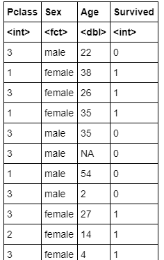
Of train.csv, only the necessary information of Pclass (room grade), Sex (gender), Age (age), Survived (survival 1, death 0) is required, so only the necessary part is extracted. Missing values are treated as'NaN', and we will proceed with the policy of removing missing values.
Reading original data, extracting data, processing missing values (source code)
import numpy as np
import pandas as pd
from IPython.display import display
from numpy import nan as NaN

titanic_train = pd.read_csv('/content/train.csv')

#Original data display
display(titanic_train)

# Pclass(Room grade)、Sex(sex)、Age(age)、Survived(Survival 1,Death 0)
titanic_data = titanic_train[['Pclass', 'Sex', 'Age', 'Survived']]
display(titanic_data)

#Missing value'NaN'Get rid of
titanic_data = titanic_data.dropna()
display(titanic_data)

#Check data to see if missing values have been removed
titanic_data.isnull().sum()
Original data reading / data extraction / missing value processing (output result)
Reading the original data

Data extraction

Missing value processing data results

Check data to see if missing values have been removed

Execution of visualization of decision tree (source code)
I'm going to use dtreeviz for visualizing decision trees with python because it's easy to see.
dtreeviz installation
!pip install dtreeviz pydotplus
Performing visualization of decision trees
import sklearn.tree as tree
from dtreeviz.trees import dtreeviz

##Convert male to 0 and female to 1
titanic_data["Sex"] = titanic_data["Sex"].map({"male":0,"female":1})

# 'Survived'Feature matrix with data looking through columns
# 'Survived'Column objective variable
X_train = titanic_data.drop('Survived', axis=1)
Y_train = titanic_data['Survived']

#Create decision tree (maximum depth of tree is specified as 3)
clf = tree.DecisionTreeClassifier(random_state=0, max_depth = 3)
model = clf.fit(X_train, Y_train)

viz = dtreeviz(
    model,
    X_train,
    Y_train,
    target_name = 'alive',
    feature_names = X_train.columns,
    class_names = ['Dead','Sruvived']
)

#Decision tree display
display(viz)
Execution of visualization of decision tree (output)

In the analysis of decision trees, it is necessary to consider how deep the tree should be analyzed. If the decision tree is not stopped at an appropriate depth, overfitting that overfits the training data used in the analysis may occur and the generalization performance may deteriorate. Due to the display this time, the maximum depth is specified as 3, so it is not set too deep, but in the teaching material, a moderate complexity parameter is specified and the tree is pruned. Since we are doing (pruning), we would like to proceed in the same way.
pruning
When looking at how well the conditional branching of each node of a decision tree is made, a parameter called impurity is often used, and the smaller this parameter is, the simpler the standard. Indicates that the classification has been completed. Another important factor involved is the complexity parameter, which indicates how complex the entire tree is. In this source code, the impureness at the time of generation of the decision tree is called Gini impureness. (DecisionTreeClassifier () argument criteria {“gini”, “entropy”}, default = ”gini”) And, as a method of generating a decision tree, we use an algorithm called Minimal cost-complexity pruning. This is an algorithm that generates a decision tree that minimizes the cost of creating a tree (number of nodes at the end of the tree x complexity of the tree + impureness of the tree), as it is called minimum cost complexity pruning. When the complexity is high, the number of nodes at the end has a strong influence on the tree generation cost, and when the decision tree is generated by the minimum cost complexity pruning, a smaller tree (smaller depth and number of nodes) is generated. I can do it. Conversely, when the complexity is low, the effect of the tree generation cost on the number of terminal nodes is small, and when generating a decision tree, a large and complex tree (small depth and number of nodes) can be generated.
I talked about a rough image without using mathematical formulas, but there are many official documents and other sites that explain in detail, so it may be a good idea to take a closer look. [Reference] https://scikit-learn.org/stable/modules/tree.html#minimal-cost-complexity-pruning
Pruning (source code)
Relationship between parameters related to complexity and parameters related to impureness
import matplotlib.pyplot as plt

#Create decision tree (no maximum tree depth specified)
clf = tree.DecisionTreeClassifier(random_state=0)
model = clf.fit(X_train, Y_train)

path = clf.cost_complexity_pruning_path(X_train, Y_train)
# ccp_alphas:Parameters related to complexity
# impurities:Parameters related to impureness
ccp_alphas, impurities = path.ccp_alphas, path.impurities

fig, ax = plt.subplots()
ax.plot(ccp_alphas[:-1], impurities[:-1], marker='o', drawstyle="steps-post")
ax.set_xlabel("effective alpha")
ax.set_ylabel("total impurity of leaves")
ax.set_title("Total Impurity vs effective alpha for training set")
Relationship between complexity parameters and the number of nodes generated and the depth of the tree
clfs = []
for ccp_alpha in ccp_alphas:
    clf = tree.DecisionTreeClassifier(random_state=0, ccp_alpha=ccp_alpha)
    clf.fit(X_train, Y_train)
    clfs.append(clf)
print("Number of nodes in the last tree is: {} with ccp_alpha: {}".format(
      clfs[-1].tree_.node_count, ccp_alphas[-1]))

clfs = clfs[:-1]
ccp_alphas = ccp_alphas[:-1]

node_counts = [clf.tree_.node_count for clf in clfs]
depth = [clf.tree_.max_depth for clf in clfs]
fig, ax = plt.subplots(2, 1)
ax[0].plot(ccp_alphas, node_counts, marker='o', drawstyle="steps-post")
ax[0].set_xlabel("alpha")
ax[0].set_ylabel("number of nodes")
ax[0].set_title("Number of nodes vs alpha")
ax[1].plot(ccp_alphas, depth, marker='o', drawstyle="steps-post")
ax[1].set_xlabel("alpha")
ax[1].set_ylabel("depth of tree")
ax[1].set_title("Depth vs alpha")
fig.tight_layout()
Pruning (output result)
Relationship between parameters related to complexity and parameters related to impureness

Relationship between complexity parameters and the number of nodes generated and the depth of the tree

In the teaching materials, pruning is performed so that the tree has a depth of about 1 to 2, so if the complexity parameter ccp_alpha is around 0.041, the depth is 1, the number of nodes is about 1, and if ccp_alpha is around 0.0151, the depth is deep. You can see that it is likely to be about 2 and 3 nodes.
Decision tree after pruning (source code)
ccp_alpha=0.041
clf = tree.DecisionTreeClassifier(ccp_alpha = 0.041)
model = clf.fit(X_train, Y_train)

viz = dtreeviz(
    model,
    X_train,
    Y_train,
    target_name = 'alive',
    feature_names = X_train.columns,
    class_names = ['Dead','Sruvived']
)

display(viz)
ccp_alpha=0.0151
clf = tree.DecisionTreeClassifier(ccp_alpha = 0.0151)
model = clf.fit(X_train, Y_train)

viz = dtreeviz(
    model,
    X_train,
    Y_train,
    target_name = 'alive',
    feature_names = X_train.columns,
    class_names = ['Dead','Sruvived']
)

display(viz)
Decision tree after pruning (output result)
ccp_alpha=0.041

ccp_alpha=0.0151

Looking at these, we can see that the biggest factor that separates life and death is gender, and women were more likely to be rescued. Even for men, the younger the age (= children), the higher the survival rate. For women, the higher the grade of the room, the higher the survival rate.
comment
The teaching materials have the following description.
Life or death of this accident The biggest factor that determines the life or death of this accident was gender. It can also be read that the crew actively rescued women and children. In addition, the superiority or inferiority of the cabin does not seem to be a factor in determining life or death.
In the result of implementing and outputting by myself, it seemed that *** the superiority or inferiority of the cabin was also a factor in determining life or death ***. The composition of the decision tree was the same regardless of whether it was python or R, so it is important not only to look at the results of the teaching materials, but also to actually execute it and analyze it in your own way. I thought.
[Reference] Implementation example and results in R (from teaching materials)
Data reading and preprocessing (R)
Reading the original data (source code)
titanic.train<-read.csv("/content/train.csv") #Specify data location str(titanic.train)
### Reading the original data (output result)

> ```console
'data.frame':	891 obs. of  12 variables:
 $ PassengerId: int  1 2 3 4 5 6 7 8 9 10 ...
 $ Survived   : int  0 1 1 1 0 0 0 0 1 1 ...
 $ Pclass     : int  3 1 3 1 3 3 1 3 3 2 ...
 $ Name       : Factor w/ 891 levels "Abbing, Mr. Anthony",..: 109 191 358 277 16 559 520 629 417 581 ...
 $ Sex        : Factor w/ 2 levels "female","male": 2 1 1 1 2 2 2 2 1 1 ...
 $ Age        : num  22 38 26 35 35 NA 54 2 27 14 ...
 $ SibSp      : int  1 1 0 1 0 0 0 3 0 1 ...
 $ Parch      : int  0 0 0 0 0 0 0 1 2 0 ...
 $ Ticket     : Factor w/ 681 levels "110152","110413",..: 524 597 670 50 473 276 86 396 345 133 ...
 $ Fare       : num  7.25 71.28 7.92 53.1 8.05 ...
 $ Cabin      : Factor w/ 148 levels "","A10","A14",..: 1 83 1 57 1 1 131 1 1 1 ...
 $ Embarked   : Factor w/ 4 levels "","C","Q","S": 4 2 4 4 4 3 4 4 4 2 ...
Data extraction (source code)
titanic.data<-titanic.train[,c("Pclass","Sex","Age","Survived")] titanic.data
### Data extraction (output result)
> 
### Missing value (NA) (source code)
> ```R
titanic.data<-na.omit(titanic.data)
Execution of visualization of decision tree (source code)
install.packages("partykit") library(rpart) library(partykit) titanic.ct<-rpart(Survived~.,data=titanic.data, method="class") plot(as.party(titanic.ct),tp_arg=T)
### Execution of visualization of decision tree (output result)
 > <img width = "480" alt = "Download (12) .png " src = "https://qiita-image-store.s3.ap-northeast-1.amazonaws.com/0/677025/4c8bf0fc-369b -137d-21b4-4c41e77c0741.png ">

### Classification tree CP (source code)

> ```R
printcp(titanic.ct)
Classification tree CP (output result)
Classification tree: rpart(formula = Survived ~ ., data = titanic.data, method = "class")
Variables actually used in tree construction: [1] Age Pclass Sex
Root node error: 290/714 = 0.40616
n= 714
CP nsplit rel error xerror xstd
1 0.458621 0 1.00000 1.00000 0.045252 2 0.027586 1 0.54138 0.54138 0.038162 3 0.012069 3 0.48621 0.53793 0.038074 4 0.010345 5 0.46207 0.53448 0.037986 5 0.010000 6 0.45172 0.53793 0.038074
### Classification tree (source code) when CP is set to 0.028

> ```R
titanic.ct2<-rpart(Survived~.,data=titanic.data, method="class", cp=0.028)
plot(as.party(titanic.ct2))
Execution of visualization of decision tree (output result)

Classification tree (source code) when CP is 0.027
titanic.ct3<-rpart(Survived~.,data=titanic.data, method="class", cp=0.027) plot(as.party(titanic.ct3))
### Execution of visualization of decision tree (output result)

 > <img width = "480" alt = "Download (14) .png " src = "https://qiita-image-store.s3.ap-northeast-1.amazonaws.com/0/677025/74101e1b-623e -94c1-40a5-8a700a5e7ec2.png ">

# Source code
 python version
https://gist.github.com/ereyester/dfb4fd6fb3e58c5d0539866f7e2622b4

 R version
https://gist.github.com/ereyester/182d5d49ea04be579da2ffc82412a82a
Recommended Posts