[PYTHON] Non-negative Matrix Factorization (NMF) with scikit-learn
NMF is a dimension reduction method and is said to be able to improve the accuracy of recommendations.
You can also easily use NMF with the Opportunity Learning Library scikit-learn.
This time, the purpose is to try it with concrete examples and understand NMF intuitively.
The article What is Matrix Factorization is easy to understand.
What is NMF
To get a rough idea of Matrix Factorization as a recommendation, it's in English, but the following materials are easy to understand. Matrix Factorization Techniques For Recommender Systems
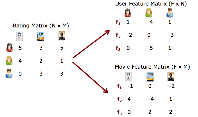
I will briefly explain the image by quoting the figure on this slide. Suppose you're assuming the Netflix Prize, where the NMF method has become so popular, and you're given a matrix that shows how many points a user and that person gave to which video (the Matrix on the left). If the user rated the video, it was rated from 1 to 5, and if it was not rated, 0 was entered. The fact that 0 is included is the heart of this problem, and we predict the true value of this 0. This Rating Matrix is decomposed into two matrices, "feature x user" and "feature x movie". Roughly speaking, NMF is a method for successful matrix factorization.
NMF formulation
\mathbf{R} \approx \mathbf{P} \times \mathbf{Q}^T = \hat{\mathbf{R}}
The error can be expressed as $ e_ {ij} ^ 2 $.
e_{ij}^2 = (r_{ij} - \hat{r}_{ij})^2 = (r_{ij} - \sum_{k=1}^K{p_{ik}q_{kj}})^2
However, the approximated $ \ hat {\ mathbf {R}} $ elements are as follows:
\hat{r}_{ij} = p_i^T q_j = \sum_{k=1}^k{p_{ik}q_{kj}}
0.5 * ||X - WH||_Fro^2
+ alpha * l1\_ratio * ||vec(W)||_1
+ alpha * l1\_ratio * ||vec(H)||_1
+ 0.5 * alpha * (1 - l1\_ratio) * ||W||_Fro^2
+ 0.5 * alpha * (1 - l1\_ratio) * ||H||_Fro^2
||A||_Fro^2 = \sum_{i,j} A_{ij}^2 (Frobenius norm)
||vec(A)||_1 = \sum_{i,j} abs(A_{ij}) (Elementwise L1 norm)
Implementation with scikit-learn
It's easy to call. For example, the code when the rating matrix is R and the feature dimension is 2 is as follows.
from sklearn.decomposition import NMF
model = NMF(n_components=2, init='random', random_state=0) # n_Specify the feature dimension with components
P = model.fit_transform(R) #Learning
Q = model.components_
Concrete example
Suppose R is a 5x4 matrix like this: The numbers in this matrix are used on this site. I referred to the example.
| D1 | D2 | D3 | D4 | |
|---|---|---|---|---|
| U1 | 5 | 3 | - | 1 |
| U2 | 4 | - | - | 1 |
| U3 | 1 | 1 | - | 5 |
| U4 | 1 | - | - | 4 |
| U5 | - | 1 | 5 | 4 |
from sklearn.decomposition import NMF
import numpy as np

#The 0 part is unknown
R = np.array([
        [5, 3, 0, 1],
        [4, 0, 0, 1],
        [1, 1, 0, 5],
        [1, 0, 0, 4],
        [0, 1, 5, 4],
        ]
    )

#Try changing the feature dimension k from 1 to 3
for k in range(1,4):
    model = NMF(n_components=k, init='random', random_state=0)
    P = model.fit_transform(R)
    Q = model.components_
    print("****************************")
    print("k:",k)
    print("P is")
    print(P)
    print("Q^T is")
    print(Q)
    print("P×Q^T is")
    print(np.dot(P,Q))
    print("R-P×Q^T is")
    print(model.reconstruction_err_ )
The output result is as follows.
****************************
k: 1
P is
[[ 0.95446553]
 [ 0.64922245]
 [ 1.12694515]
 [ 0.87376625]
 [ 1.18572187]]
Q^T is
[[ 1.96356213  1.0846958   1.24239928  3.24322704]]
P×Q^T is
[[ 1.87415238  1.03530476  1.18582729  3.09554842]
 [ 1.27478862  0.70420887  0.8065935   2.10557581]
 [ 2.21282681  1.22239267  1.40011583  3.65493896]
 [ 1.71569432  0.94777058  1.08556656  2.83382232]
 [ 2.32823857  1.28614754  1.47314     3.84556523]]
R-P×Q^T is
7.511859871919941
****************************
k: 2
P is
[[ 0.          1.69547254]
 [ 0.          1.13044637]
 [ 1.38593123  0.42353044]
 [ 1.08595617  0.3165454 ]
 [ 2.01891156  0.        ]]
Q^T is
[[ 0.          0.32199795  1.40668938  2.58501889]
 [ 3.09992487  1.17556787  0.          0.85823043]]
P×Q^T is
[[ 5.25583751  1.99314304  0.          1.45510614]
 [ 3.50429883  1.32891643  0.          0.97018348]
 [ 1.31291255  0.9441558   1.94957474  3.94614513]
 [ 0.98126695  0.72179626  1.52760301  3.0788861 ]
 [ 0.          0.65008539  2.83998144  5.21892451]]
R-P×Q^T is
4.2765298341191516
****************************
k: 3
P is
[[ 0.08750151  2.03662182  0.52066139]
 [ 0.          1.32090927  0.59992585]
 [ 0.04491053  0.44753619  3.4215759 ]
 [ 0.          0.3221337   2.75625987]
 [ 2.6249395   0.          0.91559966]]
Q^T is
[[ 0.          0.38636917  1.90213535  1.02176621]
 [ 2.62017626  1.02934221  0.          0.08629708]
 [ 0.          0.02388804  0.          1.43875694]]
P×Q^T is
[[ 5.33630814  2.14262626  0.16643971  1.0142658 ]
 [ 3.4610151   1.37399871  0.          0.97713811]
 [ 1.17262369  0.55975468  0.08542591  5.00732522]
 [ 0.84404708  0.39742747  0.          3.99338722]
 [ 0.          1.03606758  4.99299022  3.99939987]]
R-P×Q^T is
1.8626938982246695
The observation matrix R was a 5 × 4 matrix. When you try different k, you can see that P is a 5 × k matrix and Q ^ T is a k × 4 matrix.
Also, in P × Q ^ T, it is estimated that it was 0 in R. For example, when k = 2, the following $ \ hat {\ mathbf {R}} $ is completed. (The part where bold is predicted)
| D1 | D2 | D3 | D4 | |
|---|---|---|---|---|
| U1 | 5.25 | 1.99 | 0. | 1.45 |
| U2 | 3.50 | 1.32 | 0. | 0.97 |
| U3 | 1.31 | 0.94 | 1.94 | 3.94 |
| U4 | 0.98 | 0.72 | 1.52 | 3.07 |
| U5 | 0. | 0.65 | 2.83 | 5.21 |
It is a difficult problem to decide which value k should be, and it is said that it depends on the input data (R).
- Increasing k decreases R-P × Q ^ T and increases the complexity of the model.
- Conversely, if k is made smaller, R-P × Q ^ T becomes larger and the complexity of the model becomes lower.
In this case, how can we determine which k is better? (If you know, please teach)
Link
-
scikit learn reference
- http://scikit-learn.org/stable/modules/generated/sklearn.decomposition.NMF.html
-
What is Matrix Factorization (easy-to-understand qiita)
- http://qiita.com/ysekky/items/c81ff24da0390a74fc6c
-
Matrix Factorization Techniques For Recommender Systems
- https://hpi.de/fileadmin/user_upload/fachgebiete/naumann/lehre/SS2011/Collaborative_Filtering/pres1-matrixfactorization.pdf
Recommended Posts