Although not well understood in theory, it is a method of estimating a curved surface from scattered sample points. Since it is compatible with the Latin super-square sampling shown in Latin super-square sampling with OpenMDAO (scattered sampling), CAE is engineeringly used. It is often used to estimate the response surface.
The outline of the efforts is as follows. First, read the data (doe_paraboloid file) experimented with Latin super-square sampling with OpenMDAO. Next, the Kriging approximation model is trained and created using the read experimental data. Finally, the validity of the model is confirmed by plotting the interpolated value by the created Kriging approximate model as a theoretical solution (wireframe). The following equation is the theoretical solution.
\begin{align}
& f(x,y) = (x-3)^2 + xy + (y+4)^2 - 3 \\
    {\rm subject \: to} \: \: \:&  -50.0\leq x \leq 50.0 \\
                                &  -50.0\leq y \leq 50.0
\end{align}
Prepare the following training_mm.py file
training_mm.py
from __future__ import print_function
from openmdao.api import Group,  MetaModel,  FloatKrigingSurrogate

class TrainingMM(Group):
    ''' FloatKriging gives responses as floats '''

    def __init__(self):
        super(TrainingMM, self).__init__()

        # Create meta_model for f_x as the response
        mm = self.add("parabo_mm", MetaModel())
        mm.add_param('x', val=0.)
        mm.add_param('y', val=0.)
        mm.add_output('f_xy', val=0., surrogate=FloatKrigingSurrogate())
We have added a Component called MetaModel that trains an approximate model and evaluates its value. A Surrogate Model called FloatKrigingSurrogate is set to approximate f_xy. FloatKrigingSurrogate alone has the function of training the approximate model and evaluating the value. The official documentation states that MetaModel can be used to train multiple fitted models at the same time.
Prepare the following kriging_paraboloid.py. The first half is the process from reading the experimental data to training the Kriging approximate model.
kriging_paraboloid.py
#! /bin/python
import pickle
import numpy as np
import sqlitedict
from matplotlib import pyplot as plt
from mpl_toolkits.mplot3d import Axes3D
from openmdao.api import Problem
from training_mm import TrainingMM

db =sqlitedict.SqliteDict("doe_paraboloid","iterations")
res = np.array([[0.,0.,0.]] * len(db.items()))
for i, v in enumerate(db.items()):
    res[i,0] = v[1]["Unknowns"]["x"]
    res[i,1] = v[1]["Unknowns"]["y"]
    res[i,2] = v[1]["Unknowns"]["f_xy"]

prob = Problem()
prob.root = TrainingMM()
prob.setup()
prob["parabo_mm.train:x"] = res[:,0]
prob["parabo_mm.train:y"] = res[:,1]
prob["parabo_mm.train:f_xy"] = res[:,2]
prob.run()
The second half is shown below. A plot is used to compare the created kriging approximate model with the theoretical solution.
kriging_paraboloid.py continued
x = np.arange(-50., 50., 4.)
y = np.arange(-50., 50., 4.)
sg = prob.root.parabo_mm._init_unknowns_dict["f_xy"]["surrogate"]
f = open("./kriging_parabo","w")
pickle.dump(sg, f)
f.close()
f = open("./kriging_parabo_mm","w")
pickle.dump(prob.root.parabo_mm, f)
f.close()
xyzkrig = np.array([[xi,yi,sg.predict(np.array([xi,yi]))[0]] \
for xi in x for yi in y])
#xyzkrig = np.array([[0.,0.,0.]]*(25*25))
#cnt = 0
#for xi in x:
# for yi in y:
# xyzkrig[cnt,0] = prob["parabo_mm.x"] = xi
# xyzkrig[cnt,1] = prob["parabo_mm.y"] = yi
# prob.run()
# xyzkrig[cnt,2] = prob["parabo_mm.f_xy"]
# cnt += 1
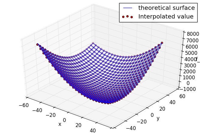
fig = plt.figure(figsize=(6,4)); ax = Axes3D(fig)
X, Y = np.meshgrid(x, y)
Z = (X-3.0)**2. + X*Y + (Y+4.0)**2. - 3.0
ax.plot_wireframe(X,Y,Z,label="theoretical surface")
ax.scatter3D(xyzkrig[:,0], xyzkrig[:,1], xyzkrig[:,2], c="r", marker="o",label="Interpolated value")
ax.set_xlabel('x'); ax.set_ylabel('y'); ax.set_zlabel('f_xy')
plt.legend()
plt.show()
The first half of kriging_paraboloid.py is omitted and only the second half is explained. First, at the beginning, we create sample points to evaluate the Kriging approximation model. This is different from the point of LHS (Latin super square sampling). The range of $ -50 \ leq x, y \ leq 50 $ is evaluated by 25 x 25 sample points divided into 25.
sg = prob.root.parabo_mm._init_unknowns_dict["f_xy"]["surrogate"]In private class variables(_init_unknowns_dict)To access,Loading surrogate model installed in Meata Model.
It's not a compliment, but there are two reasons for this.
* Saving of a trained approximation model is not implemented. This time it was serialized with pickele.
* When trying to evaluate the value of the approximate model with MetaModel, it becomes a little complicated (`` `# xyzkrig = ・ ・ ・` `` below comment line).
The rest is plotting.
The evaluation value by the Kriging approximate model is plotted with dots on the wire frame of the theoretical solution.
# Interpolation of values by Kriging approximation model
The accuracy seems to be quite good because the number of LHS samples was too large.
---