I've translated a little more about "OpenCV-Python Tutorials", so it's a useful library with OpenCV-Python bindings I also added a link to scikit-image. Both are libraries that use numpy data structures in Python, so you can use them in combination.
In the case of Scikit-image, it is provided in a form that makes it easy to link with OpenCV-Python, focusing on methods that are not provided by OpenCV-Python. Since Scikit-image supplements features that are not included in OpenCV, a wider range of image recognition technology can be realized within the framework of Python. (Sckit-Image itself does not include machine learning, machine learning is provided separately as Scikit-learn.)
The example script page in Scikit-image's Examples has a script download button. Press that button to download the script, open it in a python environment such as Spyder or IDLE, and try running it. In the scikit-image example, the data used in the example is used.
image = data.astronaut()
Because it is given in the form of, the idea of "battery included" in Python is thorough. Therefore, even beginners can execute the program without getting stuck. It's even easier to experiment with the example, as you can change the input image after you've seen it work.
### ** Common to OpenCV-Python and scikit-image **
It's exactly the same in that it uses a numpy array from within Python.
It's exactly the same that you can use matplotlib to draw graphs.
Therefore, it is exactly the same that you can display and check the matrix data used in the program with MATLAB-like output.
There is no need to write a for statement for processing matrix data for either library, and each library performs internal loop processing.
Library users are no longer aware that they are optimized.
There is no need to be aware of the difference in implementation method between OpenCV-Python and Scikit-image when using it as a library.
Since it is a Python language library, it is the same that help (function name) shows how to use the function.
### ** Did you reach the desired image processing / image recognition **?
There are methods that take different approaches for processing for the same purpose. It is encouraging that there are as many examples as possible with code and data that can actually be run.
Depending on the nature of the input data, the effectiveness of each algorithm depends on it.
One of the reasons why there are so many background removal algorithms and tracking algorithms out there is that the nature of the input data determines which one gives the best results.
At the stage of finding out which one is sufficient, trying multiple algorithms with less effort and being able to evaluate the effect of preprocessing with less processing will affect the progress of the work.
When matching the corresponding points between two images, the number of points obtained from the images varies depending on the type of feature points used. In addition, whether or not feature points can be obtained in common from two images with different fields of view (whether or not they are resistant to changes in the viewing angle) also depends on the amount of features used. As you can see, it is encouraging that scikit-image is provided with a large library of image features.
In OpenCV-Python, the tutorials are just a few of the techniques that OpenCV-Python offers. After moving the tracking in the tutorial, try a tracking technique not mentioned in the tutorial.
### ** Let's evaluate the performance **
Suppose an algorithm works well with the representative data of interest. However, it is rare that the algorithm is practical.
In practical data
・ Noise is increasing.
・ It is not bright enough.
-The image is out of focus.
-The image is distorted.
・ The white balance is out of order.
・ It is not level.
-Image resolution is low (or too high).
-The sample rate of the video is not high.
・ It is not possible to cover the diversity of subjects.
There is a possibility that the expected algorithm will fail for various reasons.
When an algorithm (including pre-processing and post-processing) that solves these problems is created, how much it can withstand the expected usage scene is determined.
### ** Let's verify the details of the algorithm while drawing a graph **
What is common to all OpenCV-Python, scikit-image, scikit-learn, "practical computer vision"
The point is that the data is visualized using [matplotlib](http://matplotlib.org/). You also need to draw a graph to see if the algorithm really gives you the results you expect. It is also necessary to visualize the progress data of what is happening in the algorithm. It is necessary to evaluate the performance, such as why this algorithm is selected and how robust this algorithm is. Graphs for such verification do not remain in the source code of the final product. Well validating them in Python will help when implementing the final product in OpenCV-C ++.
### ** Let's measure the execution speed **
e1 = cv2.getTickCount()
`# Write the code to evaluate the execution time here.
e2 = cv2.getTickCount()
timeDiff = (e2 - e1)/ cv2.getTickFrequency()
If you use the cv2 function to measure the processing time, you can measure the processing time in the same way even if the OS or CPU changes.
Whether it's OpenCV-Python or sciki-image, the Python profiler will tell you how many times the desired function is called and how much time it consumes. Python profiler is common regardless of OS type
profile.run(statement, filename=None, sort=-1)
You can do it with.
(From Spyder, it's [Run] [Profile].)
### ** Improve execution speed **
I'm running with OpenCV-Python, scikit-learn, and there are various reasons why the execution speed is slow.
-Reduce the size of the image and reduce the amount of processing.
-In multi-core, if two processes can be operated in parallel, they are operated in threads.
You can make it faster with.
[Try loading images in a separate thread](http://qiita.com/nonbiri15/items/89238c03b672c8f0579f)
[Explicitly writing a loop in numpy is extremely slow](http://qiita.com/nonbiri15/items/ef97b84832055ab807fb)
If possible, I would be happy if we could speed up the process within the framework of Python.
Are you accessing the elements of the array in a double loop against the numpy array?
Examine existing functions so you don't have to write a for loop.
There is nothing that can be used for existing functions, and I have to write a for loop.
Moreover, if you need to speed up the function, consider speeding it up by using the Cython language.
### ** When implementing in C ++ **
If your goal is not to write in C ++ and you have sufficient recognition performance and execution speed, you can stop development at that point.
(I'm happy if you're a client who says Python is enough.)
If you want a C ++ program, you will need to migrate to OpenCV-C ++ and then to OpenCV-C ++.
To migrate the algorithm verified by Scikit-Image to OpenCV-C ++, search for an implementation included in OpenCV itself in cv :: Mat type, or an implementation that performs equivalent processing using OpenCV, and port it. Will go easy. If you test with Scikit-Image whether the algorithm is enough to solve the problem you are having and finish the problem, most of the problems will be solved, so write it in cv :: Mat type. Should not bother you.
The advantage of using OpenCV-Python is that algorithms written in OpenCV-Python can be easily ported to OpenCV-C ++. In addition, you can concentrate on using and testing the algorithm without being aware of the details of what is implemented in OpenCV-Python. If you want to know the details of the algorithm, you can look at the library from OpenCV-Python, and read the C ++ source code to get further into the details.
In either case, the python interface allows you to see if the algorithm can be used for your intended use. Once you've verified, rewriting the algorithm into the OpenCV-C ++ framework should give you confidence. (Or look for an implementation of that algorithm in C ++)
Note: Both OpenCV-Python and Scikit-image are huge libraries. With this comparison, do not misunderstand that ○○ does not have △△.
### ** Scikit-image implementation approach **
In the case of Scikit-Image, the [Cython language](https://ja.wikipedia.org/wiki/Cython), which realizes speedup as a typed language while using the framework of the Python language, It will be your turn. For those who are familiar with the Python language, it will be an easy-to-understand description of the algorithm.
***
> ###** Introduction to OpenCV **
> [Introduction to OpenCV-Python Tutorial](http://docs.opencv.org/3.0-beta/doc/py_tutorials/py_setup/py_intro/py_intro.html#intro)
> Let's get started with OpenCV-Python
> [Install OpenCV-Python on Windows](http://docs.opencv.org/3.0-beta/doc/py_tutorials/py_setup/py_setup_in_windows/py_setup_in_windows.html#install-opencv-python-in-windows)
 OpenCVをwindowsで使えるようにする。
> [Install OpenCV-Python on Fedora](http://docs.opencv.org/3.0-beta/doc/py_tutorials/py_setup/py_setup_in_fedora/py_setup_in_fedora.html#install-opencv-python-in-fedora)
> Make OpenCV available on Fedora.
### ** Official information about installing Scikit-image **

[Scikit-image / Download](http://scikit-image.org/download.html)
[Installing scikit-image](http://scikit-image.org/docs/dev/install.html)
### ** Notes on installing scikit-image **
On the python interpreter
\>>> import skimage
If you don't get any errors, scikit-image is installed.
If you get an error, install it.
I will proceed only in the case of windows.
[Unofficial Windows Binaries for Python Extension Packages]
(http://www.lfd.uci.edu/~gohlke/pythonlibs/#scikit-image)
Find the compiled binary of scikit-image from.
Depending on whether the version of Python (CPython) is 2.7 or 3.x
scikit_image‑0.11.3‑cp27‑none‑win32.whl
scikit_image‑0.11.3‑cp33‑none‑win32.whl
Select the relevant Python version from the above.
Depending on whether Python is a 32-bit version or a 64-bit version
scikit_image‑0.11.3‑cp27‑none‑win32.whl
scikit_image‑0.11.3‑cp27‑none‑win_amd64.whl
Choose either.
Even if the OS version is 64bit version, python may use 32bit version. (If priority is given to the ease of library alignment, it is better to use the 32-bit version of Python and the 32-bit version of the library even on a 64-bit OS.)
To install a file with a whl extension from the windows command prompt
\> pip install filename.whl
To install.
After installation on the python interpreter
\>>> import skimage
If you don't get an error in, you know that scikit-image is successful.
***
> ###** GUI features in OpenCV **
> [Let's start image manipulation](http://docs.opencv.org/3.0-beta/doc/py_tutorials/py_gui/py_image_display/py_image_display.html#py-display-image)
画像を読み込むこと、表示すること、保存することを学びます。
> [Let's start video operation](http://docs.opencv.org/3.0-beta/doc/py_tutorials/py_gui/py_video_display/py_video_display.html#display-video)
 動画の再生、カメラからの動画のキャプチャと動画としての保存を学びましょう。
> [OpenCV drawing functions](http://docs.opencv.org/3.0-beta/doc/py_tutorials/py_gui/py_drawing_functions/py_drawing_functions.html#drawing-functions)
 直線、矩形、楕円、円などをOpenCVを使って描画することを学びます。
[Shapes いろんな形を書いてみよう](http://scikit-image.org/docs/dev/auto_examples/plot_shapes.html#example-plot-shapes-py)
The example script page in Scikit-image's Examples has a script download button. Press that button to download the script, open it in a python environment such as Spyder or IDLE, and try running it.
> [Use mouse as paint brush](http://docs.opencv.org/3.0-beta/doc/py_tutorials/py_gui/py_mouse_handling/py_mouse_handling.html#mouse-handling)
 マウスを使って塗りつぶし
> [Use Trackbar as a color palette](http://docs.opencv.org/3.0-beta/doc/py_tutorials/py_gui/py_trackbar/py_trackbar.html#trackbar)
 パラメータを制御するためのtrackbarを作る
***
> ###** Core operation **
[Basic operations on images](http://docs.opencv.org/3.0-beta/doc/py_tutorials/py_core/py_basic_ops/py_basic_ops.html#basic-ops)
>
You will learn how to read and edit pixel values, operate images in the ROI (region of interest), and other basic operations.
Sometimes you want to do the desired processing only on the ROI (area of interest) of the image.
At that time, it is important not to make the image of the area of interest a copy of the original image in order to write an efficient program.
numpy.array is a reference to a part of the original array, not a copy, when creating a subarray.
When the sub-array is rewritten, the change is automatically reflected in the original image.
There is also a way to specify a subarray for the cv :: Mat type as follows.
cv::Mat roi(img, Rect(10,10,100,100));
[Explanation of basic structure of OpenCV](http://opencv.jp/opencv-2svn/cpp/basic_structures.html)
> [Arithmetic operations on images](http://docs.opencv.org/3.0-beta/doc/py_tutorials/py_core/py_image_arithmetics/py_image_arithmetics.html#image-arithmetics)
>
Performs arithmetic operations on the image.
[Scikit-image/UsingsimpleNumPyoperationsformanipulatingimages(numpyを使って画像を扱う方法の説明)](http://scikit-image.org/docs/dev/auto_examples/plot_camera_numpy.html#example-plot-camera-numpy-py)
> [Execution performance measurement and improvement method]
(http://docs.opencv.org/3.0-beta/doc/py_tutorials/py_core/py_optimization/py_optimization.html#optimization-techniques)
> It's important to get the answer. But getting the answer the fastest is even more important. Check the speed of your code, learn to optimize your code and more.
> [Mathematical methods in OpenCV](http://docs.opencv.org/3.0-beta/doc/py_tutorials/py_core/py_maths_tools/py_maths_tools.html#mathematical-tools)
 PCA(Principalcomponentsanalysis 主成分分析)、SVD(singularvaluedecomposition 特異値分解)などのOpenCVで提供されている数学的手法のいくつかを学びます。
Translator's Note:
PCA is a method that can obtain unknown variable components and their ratios from a phenomenon in which there are many variable components. Suppose you have a large number of mixed solutions that are a mixture of multiple dyes. And suppose that the mixture is different for each lot. Suppose you have measured a number of spectra of those mixed solutions. Here's a question. How many kinds of pigments are mixed? What kind of spectrum does each of the original dyes have? How much of that dye is mixed in each mixed solution? These can be solved by a mathematical method called principal component analysis. This is an effective method for analyzing phenomena with multiple variable factors.
SVD has a lot of measurement data for determining unknown variables, and it is not possible to find unknowns by solving ordinary simultaneous equations. Such a situation actually occurs frequently. At that time, SVD (Singular Value Decomposition) is a method of finding unknowns while making use of all the data. This method should be used instead of the least squares method for analyzing experimental data. Reference information
・ [7.2 Least Squares Solution of Impossible Linear Equations](http://www.chaos.cs.tsukuba.ac.jp/ILA/doc/chapter7.pdf)
-[Calculation of simultaneous linear equations using singular value decomposition](http://sssiii.seesaa.net/article/383104769.html)
・ "Practice Computer Vision" p56 describes how to solve equations using SVD.
Unfortunately, the link to [Mathematical methods in OpenCV] has not been written yet.
***
> ###** Image processing with OpenCV **
> [Change color space](http://docs.opencv.org/3.0-beta/doc/py_tutorials/py_imgproc/py_colorspaces/py_colorspaces.html#converting-colorspaces)
 異なる色空間で画像を変換する方法を学びましょう。そして動画で色つきの物体を追跡させてみましょう。
> [Geometric transformation of images](http://docs.opencv.org/3.0-beta/doc/py_tutorials/py_imgproc/py_geometric_transformations/py_geometric_transformations.html#geometric-transformations)
 回転、変形などのさまざまな幾何変換を施してみましょう。
[Usinggeometrictransformations幾何変換を使ってみよう](http://scikit-image.org/docs/dev/auto_examples/applications/plot_geometric.html#example-applications-plot-geometric-py)
[PiecewiseAffineTransformation 画素単位のアフィン変換](http://scikit-image.org/docs/dev/auto_examples/plot_piecewise_affine.html#example-plot-piecewise-affine-py)
> [Image Threshold Processing](http://docs.opencv.org/3.0-beta/doc/py_tutorials/py_imgproc/py_thresholding/py_thresholding.html#thresholding)
 画像をグローバルしきい値、適応的閾値処理 、大津の2値化などで2値化画像に変換してみましょう。
Note: The OpenCV-Python tutorial uses numpy to explain "How Otsu's Binarization Works?". If you just show that the binarization of Otsu in OpenCV-C ++ can be used in OpenCV-Python, it is not necessary to do so, but it explains the binarization of Otsu with numpy with abundant service spirit .. The threshold () function in C ++ switches its behavior in a complicated manner depending on the argument, so it seems to be difficult to read the algorithm.
In the binarization process, what is the optimum binarization process depends on the content of the target process and the nature of the input data. In the case of dynamic binarization processing such as Otsu's binarization, it is forced to binarize, so if you give an input that you want to say "No applicable area", it may not be the expected behavior. Maybe.
[Thresholding 閾値処理](http://scikit-image.org/docs/dev/auto_examples/plot_otsu.html#example-plot-otsu-py)
[LocalOtsuThreshold 局所大津の閾値処理](http://scikit-image.org/docs/dev/auto_examples/plot_local_otsu.html)
[AdaptiveThresholding 適応的閾値処理](http://scikit-image.org/docs/dev/auto_examples/plot_threshold_adaptive.html#example-plot-threshold-adaptive-py)
> [Image Smoothing](http://docs.opencv.org/3.0-beta/doc/py_tutorials/py_imgproc/py_filtering/py_filtering.html#filtering)
 画像をぼかしたり、あつらえたカーネルを用いた画像にフィルタすることを学びます。
> [Morphological Transformation](http://docs.opencv.org/3.0-beta/doc/py_tutorials/py_imgproc/py_morphological_ops/py_morphological_ops.html#morphological-ops)
> Learn about morphological transformations such as contraction, expansion, Opening, Closing.
[MorphologicalFiltering](http://scikit-image.org/docs/dev/auto_examples/applications/plot_morphology.html#example-applications-plot-morphology-py)
[ConvexHull凸包](http://scikit-image.org/docs/dev/auto_examples/plot_convex_hull.html#example-plot-convex-hull-py)
[Skeletonize 骨格化](http://scikit-image.org/docs/dev/auto_examples/plot_skeleton.html#example-plot-skeleton-py)
[Medialaxisskeletonization](http://scikit-image.org/docs/dev/auto_examples/plot_medial_transform.html#example-plot-medial-transform-py)
> [Image Gradients](http://docs.opencv.org/3.0-beta/doc/py_tutorials/py_imgproc/py_gradients/py_gradients.html#gradients)
> 
Find image gradients, edges, and more.
[Scikit-Image/Edgeoperators エッジ操作](http://scikit-image.org/docs/dev/auto_examples/plot_edge_filter.html#example-plot-edge-filter-py)
> [Canny Edge Detection](http://docs.opencv.org/3.0-beta/doc/py_tutorials/py_imgproc/py_canny/py_canny.html#canny)
 Cannyエッジ検出を使ってエッジを見つけてみましょう。
[Scikit-Image/Cannyedgedetector Cannyエッジ検出器](http://scikit-image.org/docs/dev/auto_examples/plot_canny.html#example-plot-canny-py)
Canny edge detectors are often used when edge position accuracy is required. The following materials explain well.
[Optimal Edge Detector (Advanced Computer Vision, Wakayama University)](http://www.wakayama-u.ac.jp/~wuhy/CV05.pdf)
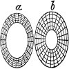
> [Image Pyramid](http://docs.opencv.org/3.0-beta/doc/py_tutorials/py_imgproc/py_pyramids/py_pyramids.html#py-pyramids)
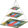 画像ピラミッドとそれを画像混合に使う方法を学びます。
[Buildimagepyramids 画像ピラミッドを作る](http://scikit-image.org/docs/dev/auto_examples/plot_pyramid.html#example-plot-pyramid-py)
> [Outline processing with OpenCV](http://docs.opencv.org/3.0-beta/doc/py_tutorials/py_imgproc/py_contours/py_table_of_contents_contours/py_table_of_contents_contours.html#table-of-content-contours)
 OpenCVにある輪郭処理の全て。
> ####** Contour processing with OpenCV **
> [Outline: Let's get started](http://docs.opencv.org/3.0-beta/doc/py_tutorials/py_imgproc/py_contours/py_contours_begin/py_contours_begin.html#contours-getting-started)
>
Find the outline and draw
> [Outline Features](http://docs.opencv.org/3.0-beta/doc/py_tutorials/py_imgproc/py_contours/py_contour_features/py_contour_features.html#contour-features)
> Learn about finding various contour features, areas, perimeters, circumscribing rectangles, etc.
Note: cv2.findContours () has side effects. Binary image given as cv2.findContours (thresh, cv2.RETR_TREE, cv2.CHAIN_APPROX_SIMPLE) The value of thresh is rewritten. If you don't want to be rewritten, it's a good idea to make a copy and give it a copy.
Rotated Rectangle is a rectangle that is closer to the contour shape.
> [Contour Properties](http://docs.opencv.org/3.0-beta/doc/py_tutorials/py_imgproc/py_contours/py_contour_properties/py_contour_properties.html#contour-properties)
> Learn to find various contour characteristics, solidity, average strength and more.
> [Outline: Other Functions](http://docs.opencv.org/3.0-beta/doc/py_tutorials/py_imgproc/py_contours/py_contours_more_functions/py_contours_more_functions.html#contours-more-functions)
>
Learn to find convexity defects, point Polygon Tests, and match with different shapes.
> [Contour Hierarchy](http://docs.opencv.org/3.0-beta/doc/py_tutorials/py_imgproc/py_contours/py_contours_hierarchy/py_contours_hierarchy.html#contours-hierarchy)
>
Learn about the hierarchy of contours.
[Contourfinding 輪郭を見つける](http://scikit-image.org/docs/dev/auto_examples/plot_contours.html#example-plot-contours-py)
> [Histogram in OpenCV](http://docs.opencv.org/3.0-beta/doc/py_tutorials/py_imgproc/py_histograms/py_table_of_contents_histograms/py_table_of_contents_histograms.html#table-of-content-histograms)
 OpenCVにあるヒストグラムの全て。
> #### OpenCV Histogram in OpenCV
[Histograms-1: Find, plot and analyze! !! !! ](Http://docs.opencv.org/3.0-beta/doc/py_tutorials/py_imgproc/py_histograms/py_histogram_begins/py_histogram_begins.html#histograms-getting-started)
> Find the histogram and draw it.
> [Histograms-2: Histogram flattening](http://docs.opencv.org/3.0-beta/doc/py_tutorials/py_imgproc/py_histograms/py_histogram_equalization/py_histogram_equalization.html#py-histogram-equalization)
> Learn to flatten the histogram to get a good contrast image.
> [Histograms --3: Two-dimensional Histogram](http://docs.opencv.org/3.0-beta/doc/py_tutorials/py_imgproc/py_histograms/py_2d_histogram/py_2d_histogram.html#twod-histogram)
> Learn to find and plot a 2D histogram.
> [Histogram-4: Histogram Backprojection](http://docs.opencv.org/3.0-beta/doc/py_tutorials/py_imgproc/py_histograms/py_histogram_backprojection/py_histogram_backprojection.html#histogram-backprojection)
> Learn to back-project a histogram on a region-colored object.
Note: In the linked OpenCV-Python tutorial example, when you give a part of the grass area from a soccer image, the corresponding color from the entire image is based on the histogram of a part of the image. It is designed to back-project the area of.
[HistogramEqualization ヒストグラムの平坦化](http://scikit-image.org/docs/dev/auto_examples/plot_equalize.html#example-plot-equalize-py)
[LocalHistogramEqualization](http://scikit-image.org/docs/dev/auto_examples/plot_local_equalize.html#example-plot-local-equalize-py)
> [Image conversion with OpenCV](http://docs.opencv.org/3.0-beta/doc/py_tutorials/py_imgproc/py_transforms/py_table_of_contents_transforms/py_table_of_contents_transforms.html#table-of-content-transforms)
 フーリエ変換、コサイン変換などOpenCVにある様々な画像変換に出会ってみましょう。
> [Template Matching](http://docs.opencv.org/3.0-beta/doc/py_tutorials/py_imgproc/py_template_matching/py_template_matching.html#py-template-matching)
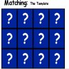 テンプレートマッチングを用いて画像中から物体を探してみましょう。
[TemplateMatching テンプレートマッチング](http://scikit-image.org/docs/dev/auto_examples/plot_template.html#example-plot-template-py)
Note: The OpenCV-Python template matching sample code shows different template matching techniques, but shows that some techniques hit something else instead of the target area. The goodness of the technique depends on the nature of the image for which template matching is used. In a world where conditions are controlled, such as machine vision, simple, low-complexity algorithms can be effective.
> [Hough Transform](http://docs.opencv.org/3.0-beta/doc/py_tutorials/py_imgproc/py_houghlines/py_houghlines.html#py-hough-lines)
 画像の中から線を検出してみましょう。
[StraightlineHoughtransform 直線ハフ変換](http://scikit-image.org/docs/dev/auto_examples/plot_line_hough_transform.html#example-plot-line-hough-transform-py)
> [Hough Transform](http://docs.opencv.org/3.0-beta/doc/py_tutorials/py_imgproc/py_houghcircles/py_houghcircles.html#hough-circles)
 画像の中から円を検出してみましょう。
[CircularandEllipticalHoughTransforms 円・楕円ハフ変換](http://scikit-image.org/docs/dev/auto_examples/plot_circular_elliptical_hough_transform.html#example-plot-circular-elliptical-hough-transform-py)
> [Image segmentation based on the Watershed algorithm](http://docs.opencv.org/3.0-beta/doc/py_tutorials/py_imgproc/py_watershed/py_watershed.html#watershed)
> Let's divide the image area using the Watershed algorithm.
[Watershedsegmentation Watershed(分水嶺)アルゴリズムの領域分割](http://scikit-image.org/docs/dev/auto_examples/plot_watershed.html#example-plot-watershed-py)
[Markersforwatershedtransform Watershed(分水嶺)変換へのマーカー](http://scikit-image.org/docs/dev/auto_examples/plot_marked_watershed.html#example-plot-marked-watershed-py)
[Randomwalkersegmentation](http://scikit-image.org/docs/dev/auto_examples/plot_random_walker_segmentation.html#example-plot-random-walker-segmentation-py)
[Findtheintersectionoftwosegmentations2種類の領域分割の積を見つける](http://scikit-image.org/docs/dev/auto_examples/plot_join_segmentations.html#example-plot-join-segmentations-py)
[Comparingedge-basedsegmentationandregion-basedsegmentation エッジベースの領域分割と領域ベースの領域分割](http://scikit-image.org/docs/dev/auto_examples/applications/plot_coins_segmentation.html#example-applications-plot-coins-segmentation-py)
[Labelimageregions 画像領域をラベリングする](http://scikit-image.org/docs/dev/auto_examples/plot_label.html#example-plot-label-py)
[Immunohistochemicalstainingcolorsseparation](http://scikit-image.org/docs/dev/auto_examples/plot_ihc_color_separation.html#example-plot-ihc-color-separation-py)
> [Interactive foreground extraction using GrabCut algorithm](http://docs.opencv.org/3.0-beta/doc/py_tutorials/py_imgproc/py_grabcut/py_grabcut.html#grabcut)
> Let's extract the foreground with the GrabCut algorithm.
***
> ###** Feature detection and feature description **
[Understanding features](http://docs.opencv.org/3.0-beta/doc/py_tutorials/py_feature2d/py_features_meaning/py_features_meaning.html#features-meaning)
 その画像の主な特徴はなんだろうか? 見つけられたこれらの特徴はどのように役に立つのか?
> [Harris Corner Detection](http://docs.opencv.org/3.0-beta/doc/py_tutorials/py_feature2d/py_features_harris/py_features_harris.html#harris-corners)
 ええ、コーナーはよい特徴? でもどうやって見つけますか?
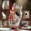
[Cornerdetection コーナー検出](http://scikit-image.org/docs/dev/auto_examples/plot_corner.html)
> [Shi-Tomasi Corner Detector and Good Features to Track](http://docs.opencv.org/3.0-beta/doc/py_tutorials/py_feature2d/py_shi_tomasi/py_shi_tomasi.html#shi- tomasi)

Let's take a look at the details of Shi-Tomasi corner detection.
> [Introduction to SIFT (Scale-Invariant Feature Transform) Features](http://docs.opencv.org/3.0-beta/doc/py_tutorials/py_feature2d/py_sift_intro/py_sift_intro.html#sift-intro)
 Harrisコーナー検出器は、画像の縮尺が変わるときには、十分良いとは言い切れません。 Loweは、縮尺に影響しない特徴を見つけるブレークスルーとなる手法を開発しました。それはSIFT特徴量と呼ばれています。
> [Introduction to SURF (Speeded-Up Robust Features) Features](http://docs.opencv.org/3.0-beta/doc/py_tutorials/py_feature2d/py_surf_intro/py_surf_intro.html#surf)
 SIFT特徴量は確かにいい特徴です。しかし、十分速いとは言えません。そこでSURF特徴量と呼ばれる高速化版が作られました。
> [FAST algorithm for corner detection](http://docs.opencv.org/3.0-beta/doc/py_tutorials/py_feature2d/py_fast/py_fast.html#fast)
 上に示した特徴検出器は全てよいものです。しかし、SLAM(訳注:SimultaneousLocalizationandMapping、自己位置推定と環境地図作成を同時に行うこと)のようなリアルタイムの用途に使えるほど十分に速いとは言えません。そこでFASTアルゴリズムの登場です。これは本当に"FAST(速い)"です。
> [BRIEF Independent Elementary Features](http://docs.opencv.org/3.0-beta/doc/py_tutorials/py_feature2d/py_brief/py_brief.html#brief)
 SIFT特徴量は、128個の浮動小数点からなる特徴記述子を用いています。そのような特徴量を数千個あつかうことを考えてごらんなさい。そのときたくさんのメモリーとマッチングのためにたくさんの時間を使
is. You can compress the features to make them faster, but you still have to calculate the features first. That's where BRIEF comes in, offering a shortcut to finding binary descriptors with less memory, faster matching, and higher recognition.
[Scikit-Image/BRIEFbinarydescriptor](http://scikit-image.org/docs/dev/auto_examples/plot_brief.html)
> [ORB (Oriented FAST and Rotated BRIEF) features](http://docs.opencv.org/3.0-beta/doc/py_tutorials/py_feature2d/py_orb/py_orb.html#orb)
 SIFT特徴量とSURF特徴量はとてもよく動くのだけれども、あなたの用途の中で使うには毎年数ドル払わなければならないとしたらどうしますか? それらは特許が成立しているのです。その問題を解決するには、OpenCVの開発者はSIFT特徴量とSURF特徴量への新しい"FREE"な代替品、ORBを思いつきました。
[Scikit-Image/ORBfeaturedetectorandbinarydescriptor](http://scikit-image.org/docs/dev/auto_examples/plot_orb.html#example-plot-orb-py)
[CENSUREfeaturedetector](http://scikit-image.org/docs/dev/auto_examples/plot_censure.html#example-plot-censure-py)
[DenseDAISYfeaturedescription](http://scikit-image.org/docs/dev/auto_examples/plot_daisy.html#example-plot-daisy-py)
[GLCMTextureFeatures](http://scikit-image.org/docs/dev/auto_examples/plot_glcm.html#example-plot-glcm-py)
[HistogramofOrientedGradients HOG特徴量](http://scikit-image.org/docs/dev/auto_examples/plot_hog.html#example-plot-hog-py)
[LocalBinaryPatternfortextureclassification](http://scikit-image.org/docs/dev/auto_examples/plot_local_binary_pattern.html#example-plot-local-binary-pattern-py)
[Multi-BlockLocalBinaryPatternfortextureclassification](http://scikit-image.org/docs/dev/auto_examples/plot_multiblock_local_binary_pattern.html#example-plot-multiblock-local-binary-pattern-py)
[Gaborfilterbanksfortextureclassification](http://scikit-image.org/docs/dev/auto_examples/plot_gabor.html#example-plot-gabor-py)
Note: The Gabor filter "[2D Gabor filter has been shown to be able to model the activity of simple cells in the early visual cortex](https://ja.wikipedia.org/wiki/%E3%82] % AC% E3% 83% 9C% E3% 83% BC% E3% 83% AB% E3% 83% 95% E3% 82% A3% E3% 83% AB% E3% 82% BF) "Wikipedia.
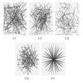
Note: When matching features, how many feature points are generated from the original image is also an important factor. Even a feature quantity that enables stable fitting with little dependence on the scale, rotation angle, and viewing angle in three-dimensional space is useless if the number of feature points generated is too small. It depends on the intended use and the nature of the input image group, so I think the appeal of the processing system including libraries such as OpenCV-Python and scikit-image is that you can easily try out a large number of features. ..
> [Feature Matching](http://docs.opencv.org/3.0-beta/doc/py_tutorials/py_feature2d/py_matcher/py_matcher.html#matcher)
 特徴検出器と記述子についてたくさん理解しました。異なる記述子を対応付ける方法を学ぶときです。OpenCVはそのために2つの手法、Brute-Forceマッチング手法とFLANNに基づくマッチング手法です。
> [Feature matching and homography for finding objects](http://docs.opencv.org/3.0-beta/doc/py_tutorials/py_feature2d/py_feature_homography/py_feature_homography.html#py-feature-homography)
 いま特徴量マッチングについて知っているので、複雑な画像中の物体を見つけるためにcalib3dモジュールとともに混ぜ合わせてみましょう。
[RobustmatchingusingRANSAC RANSACを用いたロバストなマッチング](http://scikit-image.org/docs/dev/auto_examples/plot_matching.html#example-plot-matching-py)
***
> ###** Video analysis **
> [Meanshift and Camshift Tracking](http://docs.opencv.org/3.0-beta/doc/py_tutorials/py_video/py_meanshift/py_meanshift.html#meanshift)
 私たちは既に、色に基づく追跡の例を見ました。それは単純なものです。ここでは、もっとよいアルゴリズムである平均値シフトとその改良版であるCamShiftが対象をどう見つけ追跡するのか見てみましょう。
> [Optical flow]
(http://docs.opencv.org/3.0-beta/doc/py_tutorials/py_video/py_lucas_kanade/py_lucas_kanade.html#lucas-kanade)
 重要な概念、オプティカルフローについて学びましょう。それは動画に関連していて、たくさんの用途があります。
> [Background Removal](http://docs.opencv.org/3.0-beta/doc/py_tutorials/py_video/py_bg_subtraction/py_bg_subtraction.html#py-background-subtraction)
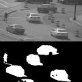 いくつかのアプリケーションでは、物体追跡のように前景を抜き出す必要があります。背景除去は、それらの場合に役立つよく知られた手法です。
***
> ###** Camera calibration and 3D reconstruction **
> [Camera Calibration](http://docs.opencv.org/3.0-beta/doc/py_tutorials/py_calib3d/py_calibration/py_calibration.html#calibration)
 利用しているカメラがどれだけ良いものか試してみましょう。それで撮影した画像に歪みが見られるでしょうか?もしあれば、どう補正しましょうか?
> [Posture estimation](http://docs.opencv.org/3.0-beta/doc/py_tutorials/py_calib3d/py_pose/py_pose.html#pose-estimation)
 calibモジュールを用いてちょっとしたかっこいい3D効果を作るのに役立つ短いセッションです。
> [Epipolar Geometry](http://docs.opencv.org/3.0-beta/doc/py_tutorials/py_calib3d/py_epipolar_geometry/py_epipolar_geometry.html#epipolar-geometry)
 エピポーラ幾何とエピポーラ制約を理解しましょう。
> [Depth distance information from stereo image](http://docs.opencv.org/3.0-beta/doc/py_tutorials/py_calib3d/py_depthmap/py_depthmap.html#py-depthmap)
 2D画像群から奥行き情報を得ます。
***
> ###** Machine learning **
> [K-nearest neighbor method](http://docs.opencv.org/3.0-beta/doc/py_tutorials/py_ml/py_knn/py_knn_index.html#knn)
 K最近傍法の使い方を学ぶとともに、K最近傍法を用いて手書きの数字認識について学びます。
> [Support Vector Machine (SVM)](http://docs.opencv.org/3.0-beta/doc/py_tutorials/py_ml/py_svm/py_svm_index.html#svm)
 SVMの考え方を理解します
> [K-means clustering](http://docs.opencv.org/3.0-beta/doc/py_tutorials/py_ml/py_kmeans/py_kmeans_index.html#kmeans-clustering)

> Learn to classify data into a group of clusters using K-means. Then you will learn to perform color quantization using the K-means method.
***
>###**Computational Photography**
Here you will learn about the various features of OpenCV related to Computational Photography, such as image denoising.
> [Image Noise Removal](http://docs.opencv.org/3.0-beta/doc/py_tutorials/py_photo/py_non_local_means/py_non_local_means.html#non-local-means)
 Non-local Meansノイズ除去と呼ばれる画像からノイズを除去する良好な手法を見ていただきます。
[Denoisingapicture](http://scikit-image.org/docs/dev/auto_examples/plot_denoise.html)
[Non-localmeansdenoisingforpreservingtextures](http://scikit-image.org/docs/dev/auto_examples/plot_nonlocal_means.html#example-plot-nonlocal-means-py)
[ImageDeconvolution](http://scikit-image.org/docs/dev/auto_examples/plot_restoration.html#example-plot-restoration-py)
> [Image Repair](http://docs.opencv.org/3.0-beta/doc/py_tutorials/py_photo/py_inpainting/py_inpainting.html#inpainting)
 たくさんの黒点とひっかきを生じた古い劣化した写真を持っていませんか?それを持ってきて、画像修復と呼ばれる方法でそれらを復元してみましょう。
[Seamcarving](http://scikit-image.org/docs/dev/auto_examples/plot_seam_carving.html)
Seam carving is an attempt to reduce the aspect ratio without adding distortion by removing less important image areas.
***
> ###** Object detection **
[Face detection using Haar cascade detector](http://docs.opencv.org/3.0-beta/doc/py_tutorials/py_objdetect/py_face_detection/py_face_detection.html#face-detection)
 Haar カスケード検出器を用いた顔検出
In the field of object detection, scikit-image provides HOG features used as a typical method for human detection.
[HistogramofOrientedGradients HOG特徴量](http://scikit-image.org/docs/dev/auto_examples/plot_hog.html#example-plot-hog-py)
Using this library, payashim ["Detecting people created with scikit-learn and scikit-image"](https://github.com/payashim/python_visual_recognition_tutorials)
Is open to the public.
***
> ###** OpenCV-Python binding **
Now let's learn how OpenCV-Python bindings are made.
> [How does the OpenCV-Python binding work? ](Http://docs.opencv.org/3.0-beta/doc/py_tutorials/py_bindings/py_bindings_basics/py_bindings_basics.html#bindings-basics)
 OpenCV-Pythonバインディングがどのように作られているのか学びましょう。
### ** How is Scikit-Image implemented? Are you **
While OpenCV is implemented in C ++, Scikit-Image is written in the Python language and the Python-based Cython language.
In a dynamically typed language, the program execution speed will be slower than in a dynamically typed language for processing to determine the type. Also, in a language that checks the range of subscripts when accessing an array element, the execution speed tends to be slow in order to ensure its security. Therefore, it is better to describe the process using a function / method that processes the array collectively, instead of the description that needs to check the range of subscripts.
[Explicitly writing a loop in numpy is extremely slow](http://qiita.com/nonbiri15/items/ef97b84832055ab807fb)
Is a description of the circumstances around that.
Therefore, based on the Python-based grammar, the Cython language is trying to speed up by simplifying the explicit type specification and checking the range of subscripts when writing a loop. .. Whether it's cv :: Mat or numpy, the idea is similar, so it's easy to move from one to the other. The following article was written by someone studying the Cython language.
[Understanding scikit-image (Cython example)](http://qiita.com/nonbiri15/items/1011eb9e658c53025e5e)
[Understanding scikit-image 2 (Cython example)](http://qiita.com/nonbiri15/items/d3643721d351eb908337)
"Cython-Speeding up Python by fusing with C" (http://www.oreilly.co.jp/books/9784873117270/)
***
A library that could not be directly supported by "OpenCV-Python Tutorials"
[NormalizedCut](http://scikit-image.org/docs/dev/auto_examples/plot_ncut.html#example-plot-ncut-py)
[RAGThresholding 領域隣接グラフ閾値処理](http://scikit-image.org/docs/dev/auto_examples/plot_rag_mean_color.html#example-plot-rag-mean-color-py)
[RAGMerging 領域隣接グラフ](http://scikit-image.org/docs/dev/auto_examples/plot_rag_merge.html#example-plot-rag-merge-py)
[DrawingRegionAdjacencyGraphs(RAGs) 領域隣接グラフを書く](http://scikit-image.org/docs/dev/auto_examples/plot_rag_draw.html#example-plot-rag-draw-py)
Above, information on comparison with scikit-image has been added to some Japanese translations of OpenCV-Python Tutorials.
Recommended Posts