[PYTHON] Miyashita's example of analytical mechanics, solved exercises and moved with animation

Miyashita I am solving an exercise in analytical mechanics. If you find any mistakes, please let us know.

Chapter 1

In the motion of a pendulum with a length of $ l $, the angle $ \ phi $ is the only substantive variable. It is more convenient to express the position of the mass point in polar coordinates instead of Cartesian coordinates. By making good use of variables that take into account binding conditions in this way, it is possible to handle substantial variables of motion.

Find the Lagrangian of the pendulum (Fig. 1.3) in Cartesian coordinates (x, y). (Example in Chapter 2 p.11)

Kinetic energy is $ T = 1 / 2m \ dot {x} ^ 2 + 1 / 2m \ dot {y} ^ 2 $, potential energy is $ U = mgy $ Therefore, Lagrangian $L=\frac{m}{2}(\dot{x}^2+\dot{y}^2)-mgy$ Also, here are the binding conditions x^2+y^2=l^2 There is.

Find the Lagrangian of the pendulum (Fig. 1.3) in polar coordinates (l, Φ). (Example in Chapter 2 p.12)

x=l\sin \phi y=-l\cos \phi Than \dot{x}=\dot{l}\sin \phi + l\dot{\phi}\cos \phi \dot{y}=-\dot{l}\cos \phi + l\dot{\phi}\sin \phi Therefore \frac{m}{2}(\dot{x}+\dot{y})^2=(\dot{l}\sin \phi + l\dot{\phi\}cos \phi)^2+(\dot{l}\sin \phi + l\dot{\phi}\cos \phi)^2=\frac{m}{2}(\dot{l}^2+l^2 \dot{\phi}^2) U=mgl\cos \phi Because $ l $ is constant L=\frac{m}{2}(l^2 \dot{\phi}^2)+mgl\cos \phi The polar coordinates handle the binding conditions well.

Equation of motion

Lagrange's equation of motion is \frac{d}{dt}\frac{\partial L}{\partial \phi}=ml^2\ddot{\phi} \frac{\partial L}{\partial \phi}=-mgl\sin \phi \therefore \ddot{\phi}=-\frac{g}{l}\sin \phi

Solving the equation of motion

Find the solution of minute vibration near Φ = 0.

When Taylor expands to the first \dot{\phi}=\frac{p_φ}{ml^2} \dot{p_\phi}=mgl\phi Will be. Therefore \ddot{\phi}=-\frac{g}{l}\phi The general solution to this equation is \phi=A\cos(\sqrt{\frac{g}{l}}t+B) If $ \ phi = \ phi_0 << 1, \ \ dot {\ phi} = 0 $ A=\phi_0, \ \dot{\phi}=A\frac{g}{l}\sin(B)=0 \therefore B=0 Therefore, \phi=\phi_0 \cos(\sqrt{\frac{g}{l}}t)

Find the solution of the vibration with Φ0 as the initial value.

\ddot{\phi_1}=-\frac{g}{l}\sin(\phi_1) Here $ \ phi_1 = \ phi + \ phi_0 $ The solution of this equation can be easily obtained by numerical analysis of Python. The second-order differential equation needs to be the first-order differential equation. \dot{\phi}=\omega \dot{\omega}=-\frac{g}{l}\sin \phi

Python uses scipy.integrate.solve_ivp. This gives the integral of the ordinary differential equation with the initial value.

scipy.integrate.solve_ivp(fun, t_span, y0, method='RK45', t_eval=None, dense_output=False, events=None, vectorized=False, args=None, **options) In

fun: function t_span: range of integration y0: initial value method:'RK45 explicit runge-tack method t_eval: Time to save the calculation result

Creating an animation

Micro vibration

%matplotlib inline 
from numpy import sin, cos
from scipy.integrate import solve_ivp
from matplotlib.animation import FuncAnimation
import matplotlib.pyplot as plt
import numpy as np

g = 9.8                                 #Gravitational acceleration[m/s^2]
l = 1.0                                 #Pendulum length[m]


t_span = [0,20]                         #Observation time[s]
dt = 0.05                               #interval[s]
t = np.arange(t_span[0], t_span[1], dt)           
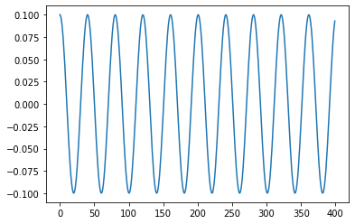
phi_0 = 0.1                              #Initial angle[deg]

phi=phi_0*cos(np.sqrt(g/l)*t)
plt.plot(phi)

x = l * sin(phi)       
y = -l * cos(phi)      

fig, ax = plt.subplots()

line, = ax.plot([], [], 'o-', linewidth=2) 

def animation(i):
    thisx = [0, x[i]]
    thisy = [0, y[i]]

    line.set_data(thisx, thisy)
    return line,

ani = FuncAnimation(fig, animation, frames=np.arange(0, len(t)), interval=25, blit=True)

ax.set_xlim(-l,l)
ax.set_ylim(-l,l)
ax.set_aspect('equal')
ax.grid()
ani.save('pendulum.gif', writer='pillow', fps=15)
plt.show()

vibration

g = 10                                 #Gravitational acceleration[m/s^2]
l = 1                                 #Pendulum length[m]

def models(t, state):#Equation of motion
    dy = np.zeros_like(state)
    dy[0] = state[1]
    dy[1] = -(g/l)*sin(state[0])
    return dy

t_span = [0,20]                         #Observation time[s]
dt = 0.05                               #interval[s]
t = np.arange(t_span[0], t_span[1], dt)
phi_0 = 90.0                              #Initial angle[deg]
omega_0 = 0.0                                #Initial angular velocity[deg/s]

state = np.radians([phi_0, omega_0])           #initial state

results = solve_ivp(models, t_span, state, t_eval=t)
phi = results.y[0,:]

plt.plot(phi)

x = l * sin(phi)       
y = -l * cos(phi)      

fig, ax = plt.subplots()

line, = ax.plot([], [], 'o-', linewidth=2) #Draw by assigning coordinates to this line one after another

def animation(i):
    thisx = [0, x[i]]
    thisy = [0, y[i]]

    line.set_data(thisx, thisy)
    return line,

ani = FuncAnimation(fig, animation, frames=np.arange(0, len(t)), interval=25, blit=True)

ax.set_xlim(-l,l)
ax.set_ylim(-l,l)
ax.set_aspect('equal')
ax.grid()
plt.show()

ani.save('pendulum.gif', writer='pillow', fps=15)

Chapter 2

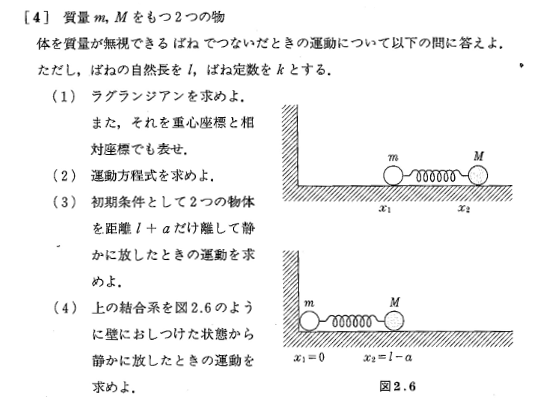
Assuming that the coordinates of the mass points are ($ x_1, y_1 ) and ( x_2, y_2 $), respectively, the kinetic energy of this system is

T=\frac{m_1}{2}(\dot{x_1}^2+\dot{y_1}^2)+\frac{m_2}{2}(\dot{x_2}^2+\dot{y_2}^2) Potential energy U=m_1gy_1+m_2gy_2 Also, the binding conditions are x_1^2+y_1^2=l_1^2, (x_2-x_1)^2+(y_2-y_1)^2=l_2^2 Is. To solve the equation of motion for Lagrangian, it is necessary to use Lagrange's undetermined constant. Therefore, we will use polar coordinates in this case as well.

x_1=l_1\sin \theta_1 y_1=l_1\cos \theta_1 x_2=l_1\sin \theta_1+l_2\sin \theta_2 y_2=l_1\cos \theta_1+l_2\cos \theta_2

Since $ l_1 and \ l_2 $ are constant, each is time-differentiated. \dot{x_1}=l_1\dot{\theta_1}\cos \theta_1 \dot{y_1}=-l_1\dot{\theta_1}\sin \theta_1 \dot{x_2}=l_1\dot{\theta_1}\cos \theta_1+l_2\dot{\theta_2}\cos \theta_2 \dot{y_2}=-l_1\dot{\theta_1}\sin \theta_1-l_2\dot{\theta_2}\sin \theta_2 Kinetic energy T_1=\frac{m_1}{2}l_1^2\dot{\theta_1}^2(\sin^2\theta_1+\cos^2\\theta_1)=\frac{m_1}{2}l_1^2\dot{\theta_1}^2 T_2=\frac{m_2}{2}[(l_1\dot{\theta_1}\sin\theta_1 +l_2\dot{\theta_2}\sin\theta_2 )^2+(-l_1\dot{\theta_1}\cos\theta_1-l_2\dot{\theta_2}\cos\theta_2 )^2] \ =\frac{m_2}{2}(l_1^2\dot{\theta_1}^2\sin^2\theta_1+2l_1l_2\dot{\theta_1}\dot{\theta_2}\sin\theta_1\sin\theta_2+l_1^2\dot{\theta_2}^2\sin^2\theta_2+l_1^2\dot{\theta_1}^2\cos^2\theta_1+2l_1l_2\dot{\theta_1}\dot{\theta_2}\cos\theta_1\cos\theta_2+l_1^2\dot{\theta_2}\cos^2\theta_2) \ =\frac{m_2}{2} (l_1^2\dot{\theta_1}^2+2l_1l_2\dot{\theta_1}\dot{\theta_2}\cos(\theta_1-\theta_2)+l_1^2\dot{\theta_2}^2) T=T_1+T_2=\frac{m_1+m_2}{2}l_1^2\dot{\theta_1}^2+\frac{m_2}{2}(2l_1l_2\dot{\theta_1}\dot{\theta_2}\cos(\theta_1-\theta_2)+l_1^2\dot{\theta_2}^2) Potential energy U_1=-m_1gl_1\cos\theta_1 U_2=-m_2g(l_1\cos\theta_1+l_2\cos\theta_2) U=U_1+U_2=-(m_1+m_2)gl_1\cos\theta_1-m_2gl_2\cos\theta_2 Therefore, Lagrangian L=T-U=\frac{m_1+m_2}{2}l_1^2\dot{\theta_1}^2+\frac{m_2}{2}(2l_1l_2\dot{\theta_1}\dot{\theta_2}\cos(\theta_1-\theta_2)+l_2^2\dot{\theta_2}^2)+(m_1+m_2)gl_1\cos\theta_1+m_2gl_2\cos\theta_2

To find Euler-Lagrangian's equation of motion \frac{\partial L}{\partial \theta_1}=-m_2l_1l_2\dot{\theta_1}\dot{\theta_2}\sin(\theta_1-\theta_2)+(m_1+m_2)gl_1\sin\theta_1

\frac{d}{dt}\frac{\partial L}{\partial \dot{\theta_1}}=\frac{d}{dt}[(m_1+m_2)l_1^2\dot{\theta_1}+m_2l_1l_2\dot{\theta_2}\cos(\theta_1-\theta_2)] \ = (m_1+m_2)l_1^2\ddot{\theta_1}+m_2l_1l_2\ddot{\theta_2}\cos(\theta_1-\theta_2)

\frac{\partial L}{\partial \theta_2}=m_2l_1l_2\dot{\theta_1}\dot{\theta_2}\sin(\theta_1-\theta_2)-m_2gl_2\sin\theta_2 \frac{d}{dt}\frac{\partial L}{\partial \dot{\theta_2}}=\frac{d}{dt}[m_2l_1l_2\dot{\theta_1}\cos(\theta_1-\theta_2)+m_2l_2^2\dot{\theta_2})] \ = m_2l_1l_2\ddot{\theta_1}\cos(\theta_1-\theta_2)+m_2l_2^2\ddot{\theta_2}

\therefore m_2l_1l_2\dot{\theta_1}\dot{\theta_2}\sin(\theta_1-\theta_2)-(m_1+m_2)gl_1\sin\theta_1 = (m_1+m_2)l_1^2\ddot{\theta_1}+m_2l_1l_2\ddot{\theta_2}\cos(\theta_1-\theta_2)

m_2l_1l_2\dot{\theta_1}\dot{\theta_2}\sin(\theta_1-\theta_2)-m_2gl_2\sin\theta_2= m_2l_1l_2\ddot{\theta_1}\cos(\theta_1-\theta_2)-m_2l_2^2\ddot{\theta_2}

Exercises p.20-21

(1) Since the force applied to the object A is $ (kx) $, the potential energy $ U = -kx ^ 2 $, the kinetic energy $ T = \ frac {1} {2} m \ dot {x} ^ 2 $ Force applied to object B $ kmg $, $ U = Mgx $, kinetic energy $ T = \ frac {1} {2} M \ dot {x} ^ 2 $

Therefore, L=\frac{1}{2}(m+M)\dot{x}^2-\frac{1}{2}kx^2+Mgx Next $ \frac{\partial L}{\partial \dot{x}}=(m+M)\dot{x}$ $ \frac{d}{dt}\frac{\partial L}{\partial \dot{x}}=(m+M)\dot{x}$ $ \frac{\partial L}{\partial x}=-kx+Mg$ The more Lagrangian equation of motion is ((m+M)\ddot{x}=-kx+Mg or (m+M)\ddot{x_1}=kx_1 (1) Where $ x_1 = -x + Mg / k $

Since the general solution of equation (1) is $ A \ sin (\ omega t + \ alpha) $ x_1=A \sin(\omega t + \alpha) (2) \dot{x_1}=\omega A \cos(\omega t + \alpha) (3)

If $ t = 0 $ $ x = 0 $, so $ x_1 = -Mg / k $, $ \ dot {x} = 0 $, so $ \ dot {x_1} = 0 $ x_1(0)=A \sin(\alpha)=-Mg/k \dot{x_1(0)}=\omega A \cos( \alpha)=0

\ cos (\ alpha) = 0 $ for $ \ omega A \ cos (\ alpha) = 0 \therefore \alpha=90^o

x_1(0)=A\sin(90^O)=A=-\frac{Mg}{k}, \therefore A=-Mg/k

\frac{\partial x_1}{\partial t} = -\omega \frac{Mg}{k} \cos(\omega t + \alpha)

x_1=-\frac{Mg}{k} \sin(\omega t+90^o) \frac{\partial x_1}{\partial t} = -\omega \frac{Mg}{k} \cos(\omega t + \alpha) \frac{\partial \dot{x_1}}{\partial t^2} = -\omega^2 \frac{Mg}{k} \sin(\omega t + \alpha)=x_1\omega^2 \ddot{x_1}=-x_1 \omega^2 Therefore, from (1) -\omega^2(m+M)x_1=-kx_1 \omega=\sqrt{\frac{k}{m+M}}

x=\frac{M}{k}g(1-\cos\sqrt{\frac{k}{m+M}}t)

(1)

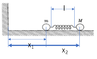
In relative coordinates

The force acting on the mass point

F=-kdx=k(l-x_2-x_1)

Potential energy

U=\frac{1}{2}k(l-x_2-x_1)^2

Kinetic energy

T=\frac{1}{2}m\dot{x_1}^2+\frac{1}{2}M\dot{x_2}^2

U=\frac{1}{2}k((l-x)^2

Will be. Therefore,

L=T-U=\frac{1}{2}m\dot{x_1}^2+\frac{1}{2}M\dot{x_2}^2-\frac{1}{2}k((l-x)^2

In barycentric coordinates

With $ X = \ frac {mx_1 + Mx_2} {m + M} $ as the center of gravity coordinates, $ x = x_2-x_1 $, $ \ dot {X} = \ frac {m \ dot {x_1} + M \ dot { x_2}} {m + M} $

\dot{X}^2=\frac{m^2\dot{x_1}^2+2mM\dot{x_1}\dot{x_2}+M^2\dot{x_2}^2}{(m+M)^2}

Because it becomes

T=\frac{1}{2}m\dot{x_1}^2+\frac{1}{2}M\dot{x_2}^2

\ \ =\frac{1}{2}(m+M)\dot{X}^2+\frac{1}{2}\frac{mM}{m+M}\dot{x}^2

Will be. Therefore

L=\frac{1}{2}(m+M)\dot{X}^2+\frac{1}{2}\frac{mM}{m+M}\dot{x}^2-\frac{1}{2}((l-x_2-x_1)^2

(2)

Lagrange's equation of motion is

$\frac{d}{dt}\frac{\partial L}{\partial \dot{x_i}} = \frac{\partial L}{\partial x_i} $

Because it is represented by

In relative coordinates

M\ddot{x_2}=k(l-x)

In barycentric coordinates

(M+m)\ddot{X}=0

\frac{mM}{m+M}\ddot{x}=k(l-x)

(3) Separating two objects by the distance $ l + a $ means $ x_2-x_1-l = a $, so if you integrate $ (M + m) \ ddot {X} = 0 $ once

\dot{X}=C

If you integrate again

X=Ct+D

Therefore, it moves linearly with the passage of time.

Also,

$ \ frac {mM} {m + M} \ ddot {x} =-k ((l-x) $ to $ A sin (wt + \ alpha) $

If $ x_3 = x-l $, then $ x_3 (t) = A sin (wt + \ alpha) $

Therefore

\dot{x_3}(t)=-w A cos(wt+\alpha)

\ddot{x_3}(t)=-w^2 A sin(wt+\alpha)=-w^2 x_3

\frac{mM}{m+M}\ddot{x_3}=\frac{mM}{m+M}(-w^2 x_3)=-kx_3

Therefore,

$w^2=\frac{k(m+M)}{mM} $

therefore

$w=\sqrt{\frac{k(m+M)}{mM}} $

x_3=A sin (wt+\alpha)

When $ t = 0 $

$ x_3 (0) = A sin (\ alpha) = 1 $ Therefore $ A = a $

$ \ dot {x_3} (0) = w A cos (\ alpha) = 0 $ Therefore $ \ alpha = 90 ^ o $

Therefore

x_3=A sin (wt+90^o)=a cos(wt)=a cos(\sqrt{\frac{k(m+M)}{mM}}t)

\because

x=a cos(\sqrt{\frac{k(m+M)}{mM}}t)+l

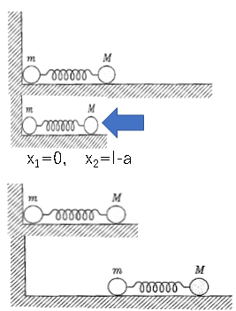
Until the mass points move away from the wall

In relative coordinates

$T=\frac{1}{2}M\dot{x_2}^2 $

U=\frac{1}{2}l(l-x_2)

Will be. Therefore

L=\frac{1}{2}M\dot{x_2}^2-\frac{1}{2}(l-x_2)

Lagrange's equation of motion is

M\ddot{x_2}=-k(x_2-l)

If $ x_3 = l-x_3 $

M\ddot{x_3}=kx_3

Therefore,

x_3(t)=A sin (wt+\alpha)

\dot{x_3}(t)=-wA cos (wt+\alpha)

\ddot{x_3}(t)=-w^2A sin (wt+\alpha)=-w^2 x_3

M \ddot{x_3}=M(-w^2x_3)=-kx_3

\because \ w=\sqrt{\frac{k}{M}}

When $ t = t_0 $

$ A sin (w t_0 + \ alpha) = a $ then $ A = a $ And $ \ alpha = \ pi / 2 $

Therefore,

w t_0 +\alpha=\pi \because t_0=\frac{\pi}{2}\sqrt{\frac{M}{k}}

After $ t_0 $, the exercise is calculated in (2). However, replace it with $ t = t-t_0 $.

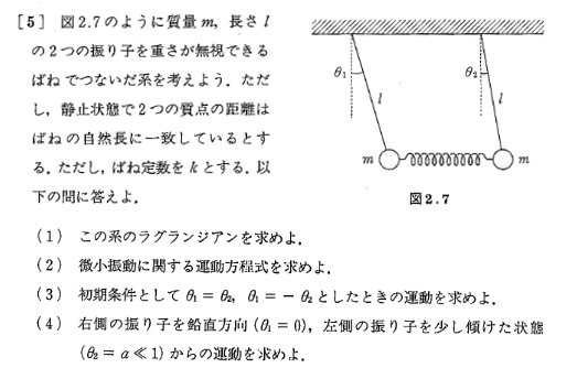
(1)

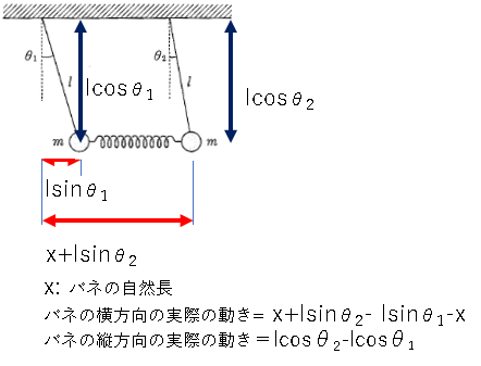
Position of mass points along the x-axis: x_1=l \cdot sin \theta_1 x_2=x+l \cdot sin \theta_2

Position of mass points in the y-axis direction: y_1=l \cdot cos \theta_1 y_2=l \cdot cos \theta_2

Therefore, the first-order time derivative is \dot{x_1}=-l \cdot cos \theta_1 \dot{\theta_1} \dot{x_2}=-l \cdot cos \theta_2 \dot{\theta_2} \dot{y_1}=l \cdot sin \theta_1 \dot{\theta_1} \dot{y_2}=l \cdot sin \theta_2 \dot{\theta_2} Therefore, the kinetic energy is $ \frac{1}{2}m(\dot{x_1}^2+\dot{x_2}^2+\dot{y_1}^2+\dot{y_2}^2)=$ $ \frac{1}{2}ml^2(\cdot cos^2 \theta_1 \dot{\theta_1}^2+\cdot cos^2 \theta_2 \dot{\theta_2}^2+ \cdot sin^2 \theta_1 \dot{\theta_1}^2+\cdot sin^2 \theta_2^2 \dot{\theta_2}^2)= \frac{1}{2}ml^2 (\dot{\theta_1}^2+\dot{\theta_2}^2)$

The potential energy of the spring U_1=\frac{1}{2}k(x_2-x_1)^2+(y_2-y_1)^2=\frac{1}{2}kl^2[(sin \theta_2-sin \theta_1)^2+(cos \theta_2-cos \theta_1)^2]

Potential energy U_2=mg(y_1+y_2)=mgl(cos \theta_1+ cos \theta_2)

Therefore, Lagrangian

L=\frac{1}{2}ml^2(\dot{\theta_1}^2+\dot{\theta_2}^2)+mgl(cos \theta_1+ cos \theta_2)-\frac{1}{2}kl^2[(sin \theta_2-sin \theta_1)^2+(cos \theta_2-cos \theta_1)^2]

(2) Since it is a minute vibration, if $ \ theta_1 <1, \ \ theta_2 <1, \ omega_g ^ 2 = g / l, \ omega_k ^ 2 = k / m $, it can be approximated as $ sin \ theta = \ theta $. From The potential energy of the spring U_1=\frac{1}{2}kl^2(\theta_2-\theta_1)^2 Also, \frac{d}{dt}\frac{\partial L}{\partial \dot{\theta_1}}=ml\ddot{\theta_1} \frac{d}{dt}\frac{\partial L}{\partial \dot{\theta_2}}=ml\ddot{\theta_2} \frac{\partial U_1}{\partial \theta_1}=-kl^2(\theta_2-\theta_1) \frac{\partial U_1}{\partial \theta_2}=kl^2(\theta_2-\theta_1) \frac{\partial U_2}{\partial \theta_1}=-mgl sin\theta_1=-mgl\theta_1 \frac{\partial U_2}{\partial \theta_1}=-mgl sin \theta_2=-mgl\theta_2 Therefore, \ddot{\theta_1}=\omega_g^2\theta_1-2\omega_k^2(\theta_2-\theta_1) \ddot{\theta_2}=\omega_g^2\theta_2+2\omega_k^2(\theta_2-\theta_1)

(3) If the initial value is $ \ theta_1 = \ theta_2 $, the two mass points move in the same direction, so add the above formulas together. \ddot{\theta_1}+\ddot{\theta_2}=-\omega_g^2(\theta_1+\theta_2) Therefore, the angular frequency is $ \ omega = \ omega_g $ If the initial value is $ \ theta_1 =-\ theta_2 $, the two mass points move in opposite directions, so the difference between the above equations is \ddot{\theta_1}-\ddot{\theta_2}=-\omega_g^2(\theta_1-\theta_2)-2\omega_k^2(\theta_1-\theta_2) Therefore, the angular frequency is $ \ omega = \ sqrt {\ omega_g ^ 2 + 2 \ omega_k ^ 2} $ Will be.

(4) Since the initial value is $ \ theta_1 = 0, \ \ theta_2 = a $, the sum of the spring angles maintains $ a $, so $ \ theta_1 + \ theta_2 = a $, and the angle difference is Keep $ \ theta_1- \ theta_2 = -a $.