[PYTHON] Implement Convolutional Neural Network

It's popular to try deep learning libraries, but even if it's okay to run Example, it often doesn't work when you try to use it in real-life cases.

I tried to move it, but the accuracy did not come out, the data processing method was bad, the model parameters were bad, I do not know the cause at all ... In order to overcome the situation, it is still necessary to understand the mechanism. I will.

That's why, in this volume, I would like to explain the steps to be taken and the reasons for it, from the very first starting line of preparing images to learning the CNN implemented in Chainer. Theory is written as the first part, but here how the parameters set in the library etc. match the theory side. I would also like to see about.

The know-how introduced this time is summarized in the following repository. I hope it will be useful when performing image recognition.

icoxfog417/mlimages

Data preparation

It is easy to think that you have to prepare a lot of data such as tens of thousands, but in recent image recognition, it is common to use a trained model.

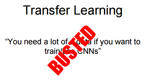CS231n Lecture11 Training ConvNets in practice, p26

Isn't the trained model only able to do "trained tasks"? As you might think (for example, cat detection), the lower layers of the model have the ability to extract the basic features of the image. Therefore, by training (or adding) only the upper layer while leaving the lower layer as it is, it is possible to obtain discrimination performance even with a small amount of data. This is called Fine Tuning (or Transfer Learning).

How many layers you should leave depends on how close your intended task is to the original "learned task".

CS231n Lecture11 Training ConvNets in practice、p33

Caffe is a well-known library for using trained models. There is an official description of the Fine Tuning method using Caffe.

Fine-tuning CaffeNet for Style Recognition on “Flickr Style” Data

Chainer can load Caffe models, so Fine Tuning is possible as well.

Personal best practices for fine tuning with Chainer

When training, if you do not want to change the value of the trained model that you have learned, you can use the volatitle flag to stop the error propagation to the trained lower layer part.

• Chainer model finetuning
• the way of fine-tuning

There is a tutorial on TensorFlow below.

• How to Retrain Inception's Final Layer for New Categories

If you want to bring a model of Caffe, there are the following tools.

ethereon/caffe-tensorflow

In this way, the number of data to be collected is gradually decreasing due to the achievements of our predecessors. This time, I have stored the trained model, so please use it (I used git lfs for the first time).

mlimages/examples

However, it can be said that it is becoming more necessary to understand what kind of model I use as a base. This point will be explained in the next section, so here we will briefly explain the acquisition of image data from ImageNet, which is famous as an image data set.

ImageNet

A dataset that tags images based on the conceptual structure of the word WordNet. The number of registered words (that is, labels) is about 100,000, and activities are being carried out with the aim of collecting about 1000 images for each word. It is also famous as the data set used in ILSVRC (ImageNet Large Scale Visual Recognition Challenge).

Now, if you are a researcher, you can download all of this dataset if you apply and get permission. If this is not the case, you will be able to get the URL of the image for each label, and you will have to drop it yourself. In addition to this, data such as image feature data and object boundaries can also be acquired.

ImageNet/Explorer

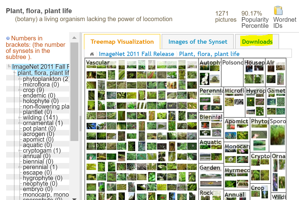
You can get the URL of the image from Download. However, there are many broken links.

I made it because it is human nature to want to download in parallel processing while avoiding broken links.

mlimages/mlimages/scripts/gather_command.py

Now, let's assume that you have downloaded and prepared the image for the time being.

Understanding the model

The collected images need to be processed according to the desired task and the trained model to be used. Therefore, here I would like to deepen my understanding by following the code of the actual model. Chainer's AlexNet code is used for explanation. This is a monumental model that started the activity of neural networks in image recognition. Note that the definition of the network is almost the same for libraries other than Chainer (Caffe, etc.), so you can think that the contents explained here can be applied to libraries other than Chainer.

chainer/examples/imagenet/alex.py

Since it is a very short code, the definition part is excerpted below.

class Alex(chainer.Chain):

    """Single-GPU AlexNet without partition toward the channel axis."""

    insize = 227

    def __init__(self):
        super(Alex, self).__init__(
            conv1=L.Convolution2D(3,  96, 11, stride=4),
            conv2=L.Convolution2D(96, 256,  5, pad=2),
            conv3=L.Convolution2D(256, 384,  3, pad=1),
            conv4=L.Convolution2D(384, 384,  3, pad=1),
            conv5=L.Convolution2D(384, 256,  3, pad=1),
            fc6=L.Linear(9216, 4096),
            fc7=L.Linear(4096, 4096),
            fc8=L.Linear(4096, 1000),
        )
        self.train = True

    def clear(self):
        self.loss = None
        self.accuracy = None

    def __call__(self, x, t):
        self.clear()
        h = F.max_pooling_2d(F.relu(
            F.local_response_normalization(self.conv1(x))), 3, stride=2)
        h = F.max_pooling_2d(F.relu(
            F.local_response_normalization(self.conv2(h))), 3, stride=2)
        h = F.relu(self.conv3(h))
        h = F.relu(self.conv4(h))
        h = F.max_pooling_2d(F.relu(self.conv5(h)), 3, stride=2)
        h = F.dropout(F.relu(self.fc6(h)), train=self.train)
        h = F.dropout(F.relu(self.fc7(h)), train=self.train)
        h = self.fc8(h)

        self.loss = F.softmax_cross_entropy(h, t)
        self.accuracy = F.accuracy(h, t)
        return self.loss

Now, if you want to customize and use it yourself, the most important are the input and output parts.

The input part is related to the size of the image and whether it should be grayscaled, and the output part is important when adding or changing the number of classes to be identified when implementing Fine Tuning. Become.

First of all, about input. The points are as follows.

• Image size: ʻinsize = 227`
• First layer to receive input: conv1 = L.Convolution2D (3, 96, 11, stride = 4)

The important thing is the definition of the first layer. According to API of Convolution2D, the setting value can be interpreted as follows.

• in_channel: 3
• out_channel: 96
• ksize: 11
• stride: 4

What do these item values represent? Here, in the theory section, [Definition of filters used for convolution](http://qiita.com/icoxfog417/items/5fd55fad152231d706c2#%E3%83%95 % E3% 82% A3% E3% 83% AB% E3% 82% BF% E3% 81% AE% E8% A8% AD% E5% AE% 9A).

• Number of filters (K): The number of filters to use. Approximately the factorial value of 2 is taken (32, 64, 128 ...)
• Filter size (F): The size of the filter used
• Filter movement width (S): Width to move the filter
• Padding (P): How much to fill the edge area of the image

First of all, a filter is like a window used for convolution. The following image determines how much the original image is compressed by this size and so on.

Then, it is easy to understand how the size of the filter determines the size after compression by looking at the figure below.

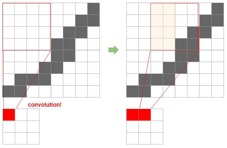
Here, a 4x4 filter is applied to an 8x8 image by sliding it by two. In this case, the final 8x8 image will be compressed to 3x3. Here, the original size is $ N $, the filter size is $ F $, the slide width is $ S $, and the compressed image width is calculated by the following formula.

If you apply this formula, you can see that $ (8 -4) / 2 + 1 = 3 $, which is exactly 3. When padding $ P $ is used to create a margin around the image (actually, the brightness is 0 = black, and in that sense, the margin is ** black **), it is as follows.

This is easy to understand by looking at the figure below, which means that the margin size x 2 is added to the original size.

As you can see from the fact that division is included, it is necessary to adjust the width of the filter to be applied, the slide width, etc. so that they are properly divisible. This is the first constraint when using other models.

I will summarize up to here. It was found that the width of the layer after applying the filter can be calculated by using the following three points out of the first points.

• Filter size (F): The size of the filter used
• Filter movement width (S): Width to move the filter
• Padding (P): How much to fill the edge area of the image

** Layer width after filtering = $ (N + P \ times 2 --F) / S + 1 $ ** ** The input image must fit the filters used in the existing model (the result of the above formula will be a good integer) **

Now, what is related to the last remaining "number of filters (K)" is the "depth (number of channels)" of the image. The number of channels is a depth element in an image and corresponds to color (RGB) in the image. Therefore, the number of channels in the first layer is often 3. On the contrary, if the existing network is used and this is 1, it means grayscale and needs to be converted to grayscale by preprocessing.

Now, let's think about what happens to the depth after folding. The depth of the filter matches the depth of the input image (otherwise it cannot be calculated), so the depth will always be "1" after convolution. Now what if we add more filters? This will increase the number of convolution layers with a depth of 1 by the number of filters (see the figure below).

Normally, CNN uses multiple filters to perform convolution in this way. In other words, the "number of filters (K)" becomes the "depth (number of channels)" after folding as it is. This is of course the same as the input depth of the next layer (I think the out_channel of conv1 and the in_channel of conv_2 have the same value in the code).

Now that we've seen all the elements of a filter, let's revisit the definition of layer 1.

• in_channel: 3-> Depth of the first image. RGB = 3
• out_channel: 96-> Layer depth after convolution = Number of filters (K)
• ksize: 11-> Filter size (F)
• stride: 4-> Filter slide width (S)

The Convolution2D also has a pad parameter, which of course corresponds to padding (P). Now you understand the parameters. And from here you can see that AlexNet has the following restrictions:

• The size of the input image must be a number divisible by 4 after subtracting 11 (the set size 227 satisfies this). * Strictly speaking, it is necessary to satisfy the definition of the following layers.
• Input image must be represented in RGB color

Therefore, the size of the image is not actually fixed, and other sizes can be used if the conditions are met. However, if you do not know whether the content learned in advance will be applied, the output part will be affected. In AlexNet, it is a linear function from the 6th layer, and from here it is the part that classifies using the convoluted result. If you do Fine Tuning, you will have to replace it or connect it to SVM, but in that case you need to understand the following definition. 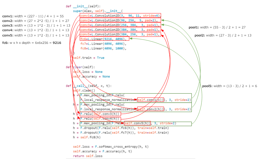The definition of the 6th layer of Chainer is fc6 = L.Linear (9216, 4096), and it is clear from this that the number of inputs is 9216 and the number of outputs is 4096, but the input "9216" Do you know what it means?

Since the output from the convolution layer is naturally "width x height x depth", it is inferred that the previous conv5 is" width x height x depth = 9216 ". The depth is clear from the fact that the out_channel of conv5 is 256, so if you divide 9216 by 256, you can see that it is 36, so width x height = 36, so the width is 6. Of course, this "6" is when the width of the input image is 227 as defined, so if you want to change the size of the input image, you need to add more and adjust the size. Of course, you can adjust the size by folding it, but you can also use pooling that adjusts the size without using weights, that is, compresses the width (see [For more information about pooling, see here in Theory](http: /). /qiita.com/icoxfog417/items/5fd55fad152231d706c2#%E3%83%AC%E3%82%A4%E3%83%A4%E6%A7%8B%E6%88%90)).

This pooling layer is also used in AlexNet, and it is because of this pooling that the width that was 13 at the stage of conv5 is now 6 at fc6. The figure below shows the calculation process up to fc6, so if you are interested, please follow it. The calculation order is conv1> pool1> conv2> pool2> conv3> conv4> conv5> pool5> fc6 (* There is no pooling between conv3> conv4 and conv4> conv5).

Therefore, if you use a large image, you should compress it a little more with this pooling (on the contrary, if it is small, it will not be pooled). As mentioned earlier, this pooling does not use weights, so the weights brought from the trained model are irrelevant. Therefore, if you use a trained model, it is better to adjust it by pooling instead of the trained and weighted convolution layer.

Finally, I would like to summarize the points when customizing the trained model. In theory, I think that this may or may not work in actual use. I would like to summarize it again as soon as I understand it.

• Layer definition reveals size and color constraints

• If you want to attach a learning machine for Fine Tuning to a specific layer, the number of inputs can be derived by calculating the size of the input image and the filter definition of each layer in order.

• Recently, it is not recommended to calculate it except for studying because it is a little complicated filtering and the layer is getting very deep. The top layer should match the number of classes to be classified, so it is recommended to attach it to the top obediently.

• If you want to resize the input image, preserve the convolution layer with the trained weights and adjust by pooling.

• Recently, it has become the mainstream not to bite Pooling, but I think that it is possible to put it in to divert the trained model.

• For "Recently" information, see Stanford Lecture (Lecture 7 p89). There is also a little bit about AlphaGo. Understanding CNN also leads to understanding how cutting-edge AI works.

Data preprocessing

At this point, I understand the model and know what kind of data should be prepared. However, what is needed when actually learning is not an "image", but a "matrix" that numerically expresses it. If you make a mistake in this conversion process, the trained model will not help. The most important points are as follows.

• Matrix transformation
• Intuitively, width (W) x height (H) x depth (K)
• If you think in a matrix, the rows of the matrix correspond to the height and the columns correspond to the width, so the matrix is H x W x K.
• When learning, it is customary to further convert this to K x H x W
• See chainer / examples / imagenet / train_imagenet.py read_image for the actual processing. ..
• Depth adjustment
• If the model assumes RGB but only brightness, duplicate the brightness value and adjust. Only brightness can be identified by the fact that the dimension is 2 (because there is no color, it is represented by a two-dimensional matrix).
• There is a format called RGBA in the world, so in this case A is dropped.
• See Caffe / io.py's load_image for the actual processing.
• Normalization of image data
• Normalize by subtracting the calculated average from all datasets. Note that, of course, all image sizes must be the same.
• See chainer / examples / imagenet / compute_mean.py for the average calculation process.
• Scaling
• RGB color and brightness take values from 0 to 255, so divide this by 255 to convert it to a value of 0-1.
• See chainer / examples / imagenet / train_imagenet.py read_image for the actual processing. ..

In the tool created this time, we implemented a class (LabeledImage) that reads an image, adjusts the depth, and then performs matrix conversion.

mlimages/mlimages/model.py

You can matrix and restore from to_array and from_array. Since the method for resizing the image is also loaded, it is possible to make a matrix after processing such as size adjustment. I hope you can use it as a reference for implementation.

The implementation is almost the same for averaging, but I tried to save it as an actual image. This makes it available even if you don't use numpy, and has the added benefit of being able to see trends in your data.

The following is an average image created from ImageNet's cat-based images, but you can see that no features are visible.

This is a bad trend. This is because if there is any feature that is common to all images, the color etc. should have changed only in that part (for a human face, the position of the eyes and mouth, etc.). Of course, if the number of images is large, it is natural that it will be blackish overall, but I think that it can be used to catch the tendency such as making it only in a certain class.

Preparation of teacher data

Well, you can't learn just by preparing images. For that image, we need to create teacher data such as which class it belongs to. This is often done in a format that is a pair of "image path" and "teacher label" (feeling below).

tabby\51879196_5a4404873a.jpg 10
tortoiseshell\1802271715_d1b3acb8f4.jpg 13
tom\1433889998_6a42ce2633.jpg 12

Of course, if you do this manually, the sun will go down, so I want to create it automatically. If the images are stored in folders for each class, the folder structure will be the teacher data as it is, so you can use this to create teacher data.

Even with the tool created this time, I made a simple script and labeled it (mlimages / mlimages / scripts / label_command.py /label_command.py)).

In addition, when images are automatically collected by scraping etc., sometimes they cannot be opened or some of them are inappropriate as teacher data. It's a good idea to eliminate those elements here, as you'll want to cry if you hit these images while learning and an exception flies and the learning that takes hours stops. When learning, it is necessary to calculate the average image for normalization (described above), and at that time, conversion and calculation to the same matrix as in production are performed, so you may check there. This time, when calculating the average image, the "image used (created) for the average calculation" is output as a file and used as training data.

Also, dividing the data into test and training data, shuffling it properly, etc. are the same as normal machine learning. This can be done simply by dividing the file or processing using random numbers, so I don't think it's too much trouble.

Model learning

Once the teacher data is ready, all you have to do is train. The biggest considerations here are performance and monitoring (though it seems to be operational management ...).

performance

For performance, the following points are important:

• GPU
• Parallel processing

GPU. I really felt this, but let's prepare a GPU machine anyway (AWS is also acceptable). With a CPU, you can't be sure that the accuracy will improve even if you wait a few days, but with a GPU, you can see it in a few hours or the calculation is completed. There are many parameters to be adjusted during training, such as model configuration, hyperparameters such as training rate, and batch size. The key is how fast this verification / confirmation cycle can be run, so it is better to solve it with hardware where it can be solved with hardware.

Compared to this, parallel processing is a device in terms of software. When learning an image, only the path to the image is written in the teacher data. Therefore, it is necessary to read the images at the time of learning, but if you do this in order from the top ..., the slow learning will be even slower, so the images in the mini-batch (a group of data to be trained at once) are parallel. It is necessary to devise such as reading with. Since multiprocessing is available in Python and ʻasyncio` is available from 3, parallelize where it can be parallelized using these modules.

Surveillance

During learning, you need to see if you are learning properly. Record the error and accuracy for each fixed amount of learning (1 batch / epoch, etc.). It is also important to save the model along the way. If you just output to the console, nothing will be left in the event of a disconnection or a lightning strike, so it is recommended to record the log file, model file, etc. in a form that remains on the disk anyway. ..

Chainer's example can be used as a reference for implementing a specific learning script.

chainer/examples/imagenet/train_imagenet.py

Since Python has become easier to write async / await from 3, I think that multiprocessing will be a little easier to write if you use Python3. I used Python3 for the tool I made this time (but there is no logging yet ...).

mlimages/mlimages/training.py/generate_batches

This completes the explanation of all the points. Finally, I will put a script that summarizes data collection, teacher data creation, and learning using it as a reference. AlexNet is used for the model as usual.

mlimages/examples/chainer_alex.py

I hope it will be helpful when you actually learn. The accuracy of this script did not improve at all on the CPU even after 2 days, but when calculated on the GPU, it became 50-60% accuracy in a few hours. In the actual model, as in the example, the accuracy does not increase while looking at it, and there is no guarantee of it. I was keenly aware that the contribution of speed is still significant in brushing up based on a legitimate evaluation of the model.