[PYTHON] Translated the explanation of the upper model of kaggle's brain wave detection competition
Not long ago, I wanted to classify brain waves using machine learning and data analysis techniques. "Grasp-and-Lift EEG Detection" that detects hand movements in kaggle competitions (https://www.kaggle.com/c/grasp-and-lift-eeg-detection) So I tried to translate it for studying. The deadline for this competition is August 2015, and from "Signal Processing & Classification Pipeline" to "Code" listed in the Github repository of Mr. Alexandre Barachant of the top team "Cat & Dog" as of February 25, 2017. I wanted to translate the section up to and the outline explanation of the model.
I am sorry that I have little knowledge about my brain and signal processing, and I have inserted "(* ~ *)" as a note to make it difficult to read. Please point out any mistakes.
Original: alexandrebarachant/Grasp-and-lift-EEG-challenge https://github.com/alexandrebarachant/Grasp-and-lift-EEG-challenge
Signal processing and classification pipeline
Overview:
The goal of this challenge is to detect six different events (* = events ) related to hand movements during grasping, lifting objects, etc. Use only brain waves ( = EEG (non-invasive) *). It is necessary to output the probabilities of 6 events in all time samples. The evaluation method is AUC (AreaUnderROCcurve) that spans 6 events.
From the viewpoint of EEG, the pattern of the brain during hand movement is characterized as a change in the spatial frequency of the EEG signal. More specifically, there should be a decrease in signal intensity in the contralateral motor cortex MU 12Hz frequency band. As the signal intensity of the ipsilateral motor cortex increases. These changes occur after the movement is performed, and some events are labeled at the beginning of the movement (eg start moving). Considering that some others are labeled at the end (such as replacing an object), it is difficult to score all 6 events with a single model. In other words, whether it is prediction or detection depends on what is classified.
The six events represent different stages of a series of hand movements (beginning to move, starting to lift, etc.). One challenge was to take into account the temporary structure of the series. That is, the continuous relationship between events. In addition, some events overlap, and some happen in a mutually exclusive manner. As a result, it is difficult to use multi-class methods or finite state machines (* automata? *) To decode sequences.
Finally, the True label is extracted from the EMG (* = EMG ) signal and given a + -150 ms frame (centered on the occurrence of the event). This 300ms has no psychological (?) Meaning. (Similar to a simple sample of 150 + 151 frames ( 301 frames *) with different labels for 150 and 151) Therefore, another difficulty was to sharpen the prediction, False Positive (= false positive) To minimize (at the edges of the frame).
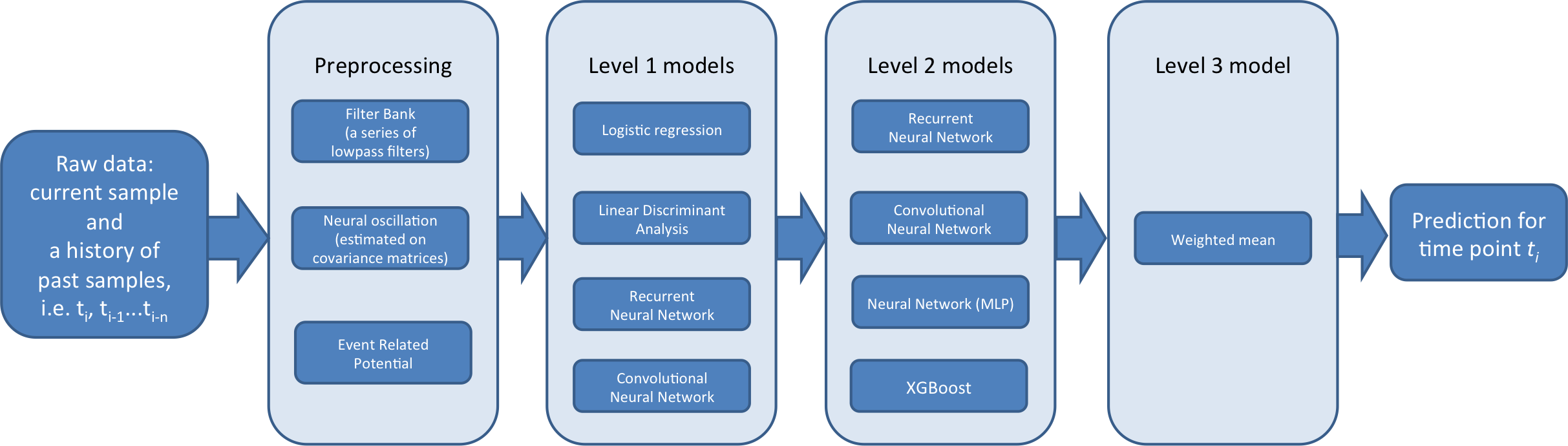
In such a context, create a three-level classifier pipeline:
--Lvl1 is subject-specific. That is, each subject is trained individually. Many of them are also event-specific (* that is, it seems that many subjects have only one movement ). The main goal of Lvl1 is to provide support and versatility for Lvl2 modules. By embedding subjects and events with different types of features. ( Level 1 outputs a new feature from the feature and sends it to the level 2 classifier in the subsequent stage *)
--Lvl2 is a global model (not patient-specific). Trained on the results of Level 1 predictions (meta-features). Their main goal is to consider the temporary structure between events. Also, the fact that they help correct predictions among subjects significantly globally (* is *).
--Lvl3 is an ensemble of predictions for Lvl2. It goes through an algorithm that optimizes the weight of 2 to maximize the AUC. This step improves the sharpness of predictions, avoiding overfitting.
No future data rules
We paid close attention to the causal relationship. A temporary filter is applied at all times, but I used the lFilter function (Scipy). It is a function that implements "direct form II causal filtering". A sliding window is used at each time, but we padded the signal with zeros on the left. The same idea applies when the history of past forecasts is used. (Same idea was applied when a history of past prediction was used) Finally, since the signal or prediction was concatenate across the unprocessed time series, the last sample of the previous series can "leak". This is not a rule violation. Because the rules apply only in a particular time series.
Model description
Here is an overview of the 3-level pipeline
Lvl1 The model is described as follows. Trained with raw data in validation mode and test mode (?). The previous model was trained in series 1-6 and the predictions were 7-8 (these predictions are level 2 training data (meta-features). Later modes are trained on series 1-8 and predicted on test series 9-10. (* 9-10 is the prediction target to be submitted, learns 1-6 for it, and outputs the prediction of 7-8. After that, it means that the prediction is output as input and the prediction of 9-10 is output by Lvl2. ? *)
Cov The covariance matrix is a feature of selection for detecting hand movements from brain waves. They contain spatial information (through per-channel covariance) and frequency information (through signal distribution). The covariance matrix is predicted in a sliding window (usually 500 samples). After using a bandpass filter to the signal. There are two types of covariance:
-
1.AlexCov: The event label is first relabeled. To a series of 7 states. For each brain state, the geometric mean (* described later *) corresponding to each covariance matrix is estimated. (By calculating the LOG Euclidean metric) After that, while creating a size 7 feature vector, the Lehman distance to each center of gravity is calculated. This procedure can be regarded as a supervised manifold embedding with a Riemannian metric using Riemannian metric. (?)
-
2.RafalCov: Same idea as above, but applied separately for each event. While creating a 12-element feature vector (There are 2 classes, 1 and 0, for each event)
ERP (* Event-related potential, ERP) ) This dataset contains a visually evoked potential (related to the experimental paradigm). The features for asynchronous ERP detection are basically based on what was done in the previous BCI challenge ( the author has previously worked on the ERP detection challenge *). During training, the signal is epoched 1 second before the start of each event. ERP was averaged and reduced using the Xdawn algorithm (before being combined with an established signal). Then the covariance matrix was inferred and processed. Similar to the covariance feature.
FBL The signal was found to contain a lot of predictive information. At low frequencies. Therefore, we will introduce the filter bank method. It consists of combining the results of applying several 5th order Butterworth lowpass filters. (Cutoff frequencies are 0.5, 1, 2, 3, 4, 5, 7, 9, 15, 30 Hz)
FBL_DELAY The FBL, however, has a single raw data / observation of 2 seconds together with 5 past samples (1000 samples in the past, each taking only the 200th sample?). It is extended by spanning it into an interval. These additional features allow the model to capture the temporary structure of the event.
FBCL The filter bank combines the features of the covariance matrix together into a feature set.
algorithm
** Logistic Regression **, ** LDA (Linear Discriminant Analysis) ** Different standardizations are applied to testing and pre-training) Under the above characteristics, an event-specific perspective? Is provided on the data?
There are also two LVL1NN methods, neither of which is event specific. (All events are learned at the same time) (following)
Convolutional Neural Network This is a family of models (based on Tim Hochverg's script and Bluefool's tweaks. [Tim Hochberg's script with Bluefool's tweaks](https://www.kaggle.com/bitsofbits/grasp-and- lift-eeg-detection / naive-nnet): Lowpass filter and option 2dCONV (It spans all electrodes, so each filter captures dependencies between all electrodes at the same time.) In summary, this is a small 1D / 2D convolutional NN (input → dropout → 1d / 2dConv → dense → dropout → dense → dropout → output) Like being learned with some of the current and past samples. Each CNN is tagged 100 times to reduce the relatively high variance (* variability ) between each run ( Bagging ?, see below *), Is that one run caused to take advantage of an efficient epoch strategy that trains the network with a random portion of the training data? Something like.
Recurrent Neural Network A small RNN trained on the signal after passing through a lowpass filter (input-> dropout-> GRU-> dense-> dropout-> output)) (Filter bank of low-pass filter and cutoff frequency of 1, 5, 10, 30hz) Trained in a short, sparse time series change of 8 seconds (take each 100th sample up to the last 4000 samples). RNNs seem to be perfectly applicable to this task (a well-defined temporary structure of events and their intermediate dependencies (* interdependencies, co-occurrence? *)), But in practice they get good predictions. Was hard. Therefore, the calculation cost was high, so I didn't pursue it as much as I expected.
Level2 These models are trained with the output of level 1 models. They are trained in Validation and Test modes. Validation is a cross-validation method that is performed, dividing each series (2 folds (* group *)). The predictions from each fold are then metafeatured (this is what we call the new features transformed using the model), for the Lvl3 model. This test mode model is trained in series 7 and 8 and the predictions are output for test series 9 and 10.
algorithm
XGBoost Gradient boosting machines provide a unique perspective on the data, achieve very good scores, and bring diversity to the next stage of the model. Only Lvl2 is trained individually for each event, and the subject ID is added as a feature. It helps correct predictions between subjects (adding one-hot encoding of subject IDs does not improve performance in NN-based models). XGBoost correctly predicts a particular event, this accuracy is very good when trained with a few seconds of time series signals, not just the corresponding event, but the meta-features of all events. Because they extract predictive information contained in intermediate dependencies between events and related transient structures. Furthermore, if you work hard on the input subsamples, you can standardize them and prevent overfitting.
Recurrent Neural Network A very high AUC can be achieved with a well-defined temporary structure of events and a variety of Level 2 metafeatures. Training with Adam has a low computational cost (in many cases it only takes one epoch to converge). The large number of Level 2 models is a simple RNN architecture with minor modifications (input-> dropout-> GRU-> dense-> dropout-> output), which is a subsampled short time course of 8 seconds (* timecourse). , Time series change, input data length? *).
Neural Network Trained in a small multi-layer (only one hidden layer) subsampled 3-second history time series. This was worse than RNNs and XGBoost. But it provided versatility for the Lvl3 model.
Convolutional Neural Network Small Lvl2 CNNs (one convolutional layer, no pooling, then one dense layer) are trained in a 3-second subsampled history timecourse. A filter that spans all predictions and strides for a single time sample is created between the time samples. For multilayer NNs, the main purpose of these CNNs is to provide versatility for the Lvl3 model.
The versatility of the Lvl2 model is extended by running the above algorithm with the following modifications:
--Make meta features into different subsets --Change the length of the time course history --Log sample history (* Make time series sample log? *) (Recent time points are sampled more closely than even interval sampling) --bagging (see below)
For NNs, CNNs, RNNs:
--Use parametric ReLu instead of Relu for activation function of dense layer --Multi-layer --Change the optimizer (SGD or ADAM)
Quoted from Toki no Mori Wiki http://ibisforest.org/index.php?%E3%83%90%E3%82%AE%E3%83%B3%E3%82%B0
Bagging †
A method of synthesizing discriminators generated by repeating bootstrap sampling to generate discriminators with higher discrimination accuracy. The name comes from Bootstrap AGGregatING
In the field of neural networks, it is also called a committee machine.
Bootstrap sampling †
How to create a new sample set X'from the sample set X = {xi} N by allowing duplication and sampling
Bagging Some models are additionally tagged. To increase its robustness. Two types of bagging are used:
--Select a random subset from the training targets. For each Bag (model contains multiple Bags in its name) (* filename in the author's repository ) --From the meta-features of choosing a random subset, for each bag (named bags_model) ( filename in the author's repository *)
Found 15 Bags in all cases (* run? *) To get satisfactory results. AUC does not increase much even if it is increased further.
Level3 Lvl2 predictions are ensembled. Through an algorithm that optimizes ensemble weights to maximize AUC. This step increases the sharpness (accuracy?) Of the prediction, and using a very simple ensemble technique prevents overfitting. (It was a threat to the (* = overfitting ) actually advanced ( high Lvr, = many stages? *) Ensemble.) To further increase AUC and to increase robustness. We used three weighted averages for:
--Arithmetic mean (* ordinary average )
--Geometric mean ( Multiply each and take the root *)
--Index average:
f
The Lvl3 model is the average of the above three weighted averages.
Submission
| Submission name | CV AUC | SD | Public LB | Private LB |
|---|---|---|---|---|
| "Safe1" | 0.97831 | 0.000014 | 0.98108 | 0.98095 |
| "Safe2" | 0.97846 | 0.000011 | 0.98117 | 0.98111 |
| "YOLO" | 0.97881 | 0.000143 | 0.98128 | 0.98109 |
Safe1 A cross-validated model with a relatively high AUC and stability was used as the final submission (lvl3) model. Robust metafeatures of lvl2 (7/8 of lvl2 model is Baged)? (7 out of 8 level2 models were bagged.)
Safe2 Another submission that is a very stable CV (* cross-validation? *) AUC. This Lvl2 meta feature (only 6/16 bag)? (only 6 level2 models out of 16 were bagged) was considered to be a less secure choice for Lvl2 than safe1 (wrongly (?)) And was not actually chosen in the final submission. I'm just interested here.
YOLO (* YOLO, meaning "life is only once"? *) The second final submission is the average of 18 Lvl3 models. Meaning them together results in increased robustness. Of CV and public LB scores in cross-validation. This submission is a bit overfitted and you can avoid its high computational costs by running either Safe1 or Safe2. Both output similar AUCs on private leaderboards.
Discussion
Are you actually decoding the activity of the brain?
Based on a wide range of features, it is unclear whether these models actually decode brain activity related to hand movements. By using complex preprocessing (due to covariance features) or the black box algorithm (CNN) poses additional difficulties. When analyzing the results. (* Is it the story of the problem that the result of NN cannot be explained why it happened? *)
The good performance of models based on infrequent features raises further doubts. These features are not known to be particularly useful in decoding hand movements. More specifically, it is very difficult to obtain good results by detecting an event having a frequency of 1 Hz or less and 300 ms. The explanation changes when the baseline (* basic waveform data? ) Changes due to the movement of the torso, or when the subject touches an object and touches the ground. ( I understand that it means that it can be detected in such cases *)
Also, with a covariance model that predicts in the 70-150hz frequency band, where relatively good performance can be observed. This frequency band contains a lot of EEG (* = EEG *), and the activity of EMG related to the task is latent.
- EMG (electromyography --EMG) *
But the dataset is very clean and contains strong patterns related to the event, which is this [script](https://www.kaggle.com/alexandrebarachant/grasp-and-lift-eeg-detection/common- You can see it in spatial-pattern-with-mne). Other activities (VEP *, EMG *, etc.) may contribute to overall performance, by forcing predictions in more difficult cases (re-enforcing predictions for harder cases), but in fact we Is undoubtedly decoding brain activity related to hand movements.
- Visual evoked potentials (VEP) are potentials generated in the visual cortex of the cerebral cortex by giving visual stimuli (from Wikipedia) *
Do you need all these models?
In this challenge I made great use of the ensemble. The problem with this method (prediction of all samples) was devoted to this kind of solution. (?) (The way the problem was defined (prediction of every sample) was playing in favor of this kind of solution), In such a situation, increasing the number of models always improves the performance and the prediction accuracy.
In a real application, it is not necessary to classify all time samples, and one time frame method is used, for example, output every 250ms. I believe it is possible to get equal decoding performance with a more optimal solution, by stopping the ensemble at Lvl2 and using only a subset of some Level 1 models. (One for each type of feature).
Recommended Posts