Recently, I'm interested in dealing with music by machine learning, and I've been researching various things, but since it's a big deal, I'll write an article that serves as a memorandum and promotes understanding.

Not limited to machine learning, when treating music as digital information, it is roughly divided into a method of handling meta information such as sheet music, tones, lyrics, and a method of handling audio data itself, but this time the audio data itself is treated. As one of the methods to handle, I will summarize MFCC.

For those in a hurry

Make mp3 wav and MFCC to drop it to a dimension that can be handled realistically

#Install ffmpeg
$ brew install ffmpeg
#Sampling mp3 with ffmpeg rate 44.Convert to 1kHz wav
$ ffmpeg -i hoge.mp3 -ar 44100 hoge.wav
#Install the required Python packages
$ pip install --upgrade sklearn librosa

# python
import librosa
x, fs = librosa.load('./hoge.wav', sr=44100)
mfccs = librosa.feature.mfcc(x, sr=fs)
print mfccs.shape
# (n_mfcc, sr*duration/hop_length)
#The dimension of the coefficient obtained after DCT(Default 20) ,Sampling rate x audio file length (=Total number of frames)/STFT slide size(Default 512)

mfccs is a nice dimensional ndarray.

For those who are not in a hurry

As mentioned at the beginning, there is a motivation to handle audio data with machine learning logic, but for example, with the sound quality commonly called "CD sound quality", it was recorded for 1 second in an uncompressed format called linear PCM. If the data size is

CD sound quality-Sampling rate 44.1kHz, bit depth 16bit, stereo 44,100 (Hz) x 16 (bit) x 2 (ch / stereo) ~ 1,411 (kbps)

Therefore, 10 seconds of data will be about 1.2MB in size. Even if it is made monaural and one frame is represented by float, it is 4.4 x 10 ^ 5 dimensions in 10 seconds. Kittsu. Therefore, it is necessary to reduce the information as voice to a level that can be handled realistically without abundant computing resources like Google, but as a typical method, MFCC (Mel-Frequency) is required. Introducing Cepstrum Coefficients.

What is the Mel frequency cepstrum coefficient?

It is the coefficient of "Cepstrum" of "Mel frequency". I don't know what it is yet, so let's take a look at each one.

What is a mel (scale) frequency?

The mel scale (Mel scale, English: mel scale) is a perceptual measure of pitch. If the difference in the mel scale is the same, it is intended that the difference in pitch felt by humans will be the same. -Mel Scale-Wikipedia

So, it's a scale that takes into account human pitch perception. It seems that there are many things that are not known about human pitch perception, but it seems that sounds near the lower limit of the audible range are heard higher, and sounds near the upper limit are heard lower. The mel scale is based on 1000 mel = 1000 Hz and is calculated by the following formula.

m = m_0 \ln{(\frac{f}{f_0}+1)}

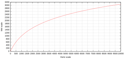
It's slowly increasing in the high register.

$ f_0 $ is an expression derived from the constraint of $ 1000 mel = 1000 Hz $ $ m_0 = \frac{ 1000 }{ \ln { \frac{1000}{f_0} + 1 }} $

It is a parameter calculated by. As an example, the conversion to the Mel scale is calculated as follows:

m = 1125 \ln{(\frac{f}{700} + 1)}

From 1000 mel, the height is doubled to 2000 mel and halved to 500 mel. Note that from the above formula, it is different from the octave (double the frequency) in the frequency domain.

What is cepstrum

A cepstrum is a Fourier transform of the logarithm (phase unwrapped) of the Fourier transform (of a signal). Also called the spectrum of the spectrum. It is common to explain the processing process as FT → log → IFT (Inverse Fourier Transform). That is, cepstrum is defined as "the inverse Fourier transform of the logarithm of the spectrum". This is not the definition in the original paper, but it is widely used. -[Cepstrum-Wikipedia](https://ja.wikipedia.org/wiki/%E3%82%B1%E3%83%97%E3%82%B9%E3%83%88%E3%83%A9% E3% 83% A0)

It's a little difficult, but after Fourier transforming the audio signal as waveform data and converting it to a frequency spectrum, the logarithmic value is inverse Fourier transformed and returned to time and space. Cepstrum analysis-A breakthrough on artificial intelligence As detailed here, the spectral fine structure (fine movement) and envelope in the logarithmic spectral region It seems that you are happy that the structure (gradual change) can be separated.

Conversion procedure

I have somehow imagined that MFCC would seek "cepstrum" in the "mel frequency domain", so I would like to take a look at the specific procedure for finding MFCC from audio signals. (Since MFCC is a "mel frequency cepstrum coefficient", it seems that the name refers to the value after conversion processing, but even if you look at papers etc., it seems that this name is used as the conversion processing itself. Therefore, I hope that you can interpret it as the conversion process itself according to the context as appropriate.)

It seems that there are various sub-streams of MFCC calculation method itself, but this time I referred to the following.

Beth Logan(2000), Mel Frequency Cepstral Coefficients for Music Modeling

It describes the adaptation of MFCC to music modeling, which is used as a feature of speech recognition.

Also, for the specific calculation method

-Mel Frequency Cepstrum Coefficient (MFCC)-A Breakthrough on Artificial Intelligence -Note on MFCC calculation method -Mel Frequency Cepstrum (MFCC)-Miyazawa ’s Pukiwiki

The mel frequency scale and coefficients

I am also familiar with the area.

The procedure described in the paper is as follows.

Divide the audio data into frames of appropriate length
Apply the Window function and perform discrete Fourier transform to obtain the frequency spectrum.
Take the logarithm
Collect and smooth BINs evenly at the mel frequency
Discrete cosine transform

Let's take a closer look.

1,2. Frame division ~ Window function adaptation ~ Discrete Fourier transform

This is STFT (Short-term Furier transform), isn't it?

Short-time Fourier transform (Tanjikan Fourier transform, short-time Fourier transform, short-term Fourier transform, STFT) is to multiply a function by shifting the window function and then perform the Fourier transform. [Short-time Fourier transform-Wikipedia](https://ja.wikipedia.org/wiki/%E7%9F%AD%E6%99%82%E9%96%93%E3%83%95%E3%83% BC% E3% 83% AA% E3% 82% A8% E5% A4% 89% E6% 8F% 9B)

STFT in discrete time

STFT_{x,w} [n,\omega]=\sum_{m=-\infty}^{\infty} x[n+m]w[m]e^{-i \omega m}

Here, $ w [m] $ is a window function, the center is a value near 1, and it is a function that converges to 0 outside the range. Multiply by the target function for the purpose of smoothing both ends. The Hamming Window, which is also used in this paper and is often used, has the following form.

Window function-Wikipedia

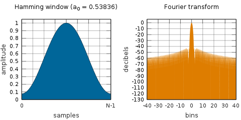
Usually the absolute value is squared to get the power spectrum (it adapts to all the divided frames, so you get the time variation). The phase information will be lost, but as the paper says, the amplitude information is more important than the phase information, so let's say it is good.

3, 4. Smoothing in the Mel frequency band

The image looks like this.

Although not specified in the paper, this is usually calculated by applying a "mel filter bank". A mel filter bank is a bandpass filter (a filter that extracts only a specific frequency band) at regular intervals in the mel frequency domain, and has the following shape.

The mel frequency scale and coefficients

Details on how to make a mel filter bank are as follows.

Mel Frequency Cepstral Coefficient (MFCC) tutorial

As an example, create a mel filter bank that divides the frequency band from 300Hz to 8000Hz into 10 subbands by the following procedure.

Convert the lower and upper limits of 300Hz and 8000Hz to mel frequencies $ (300Hz, 8000Hz) = (401.25 Mel, 2834.99 Mel) $ 2.1) Divide the above area (10 + 2) $ m(i) = [401.25, 622.50, 843.75, 1065.00, 1286.25, 1507.50, 1728.74, 1949.99, 2171.24, 2392.49, 2613.74, 2834.99]Mel $ 3.2) Return to frequency $ h(i) = [300, 517.33, 781.90, 1103.97, 1496.04, 1973.32, 2554.33, 3261.62, 4122.63, 5170.76, 6446.70, 8000]Hz $
Define the mth filter below

H_m(k)=\begin{cases}
    0 & k < h(m-1) \\
    \frac{ k - h(m-1) }{ h(m) - h(m-1) } & h(m-1) \leq k \leq h(m) \\
    \frac{ h(m+1) - k }{ h(m+1) - h(m) } & h(m) \leq k \leq h(m+1) \\
    0 & k > h(m+1) \\
  \end{cases}

At each frame, this filter is applied to the logarithmic BIN power, and the sum of each subband m is used as the input signal for the next step.

5. Discrete cosine transform (DCT)

DCT transforms a finite sequence into a coefficient of a linear combination (that is, the sum of the appropriate frequency and amplitude cosine curves) based on the cosine function sequence cos (nk). In DCT, the coefficient becomes a real number and the degree of concentration on a specific component increases. It is used in a wide range of applications such as image compression such as JPEG, audio compression such as AAC, MP3, and ATRAC, and digital filters. [Discrete Cosine Transform-Wikipedia](https://ja.wikipedia.org/wiki/%E9%9B%A2%E6%95%A3%E3%82%B3%E3%82%B5%E3%82%A4 % E3% 83% B3% E5% A4% 89% E6% 8F% 9B)

In short, let's express a certain signal sequence by adding cosine waves of various amplitudes and phases. When I hear that much, I wonder what is different from DFT, but as you can see in ↑, there is no imaginary part unlike $ e ^ {-iω} $, so I'm glad that you can always get a real number if you enter a real number. When.

It seems that there are various basis functions, but taking DCT-II, which is often used in Wikipedia, as an example, for $ f_i $ with N data, the basis functions

\phi_k[i] = \begin{cases}
  \frac{ 1 }{ \sqrt[]{N} } & k=0 \\
  \sqrt[]\frac{ 2 }{ N } \cos \frac{ (2i + 1)kπ }{ 2N } & k=1,2,...,N-1 \\
  \end{cases}

Using,

C[k] = \sum_{i=0}^{N-1}f_i\phi_k[i]

Ask as. The feature of DCT is that the information is concentrated on a small number of low frequency components, so it is possible to compress the dimensions while leaving as much information as possible by cutting off the information from the lower order term by an appropriate number. So, if you DCT the discrete signal obtained in the previous calculation and take the low-order term, you can get the MFCC congratulations!

Implementation example in librosa

As we saw at the beginning, using librosa you can get (!) MFCC in just one line by opening a wav file. Since it is a great deal, I would like to visualize the calculation progress while looking at the implementation.

The code is based on the following. I ran it on Jupyter.

Notes on Music Information Retrieval

setup

To run the following code, you need to have python and jupyter installed as a preliminary preparation. For Mac users, it is recommended to install anaconda from pyenv via anyenv. Also,

http://musicinformationretrieval.com/python_basics.html

Execute the command in Package Installation to install the required libraries. You should be able to complete the setup by hitting the following command innocently. Python is 2.7.

$ brew install anyenv
$ anyenv install pyenv
$ pyenv install anaconda2-4.3.0
$ pip install --upgrade sklearn librosa seaborn mir_eval matplotlib
$ ipython notebook

Implementation

Now for the implementation code. First, download the sample wav file and plot the waveform.

%matplotlib inline
import matplotlib.pyplot as plt, librosa, librosa.display, urllib

#Download sample file
urllib.urlretrieve('http://audio.musicinformationretrieval.com/c_strum.wav', './c_strum.wav')
x, fs = librosa.load('./c_strum.wav', sr=44100)
librosa.display.waveplot(x, sr=fs, color='blue')

Since the function to get MFCC is prepared, it can be converted only with the following code as introduced at the beginning.

#mfcc and plot
mfccs = librosa.feature.mfcc(x, sr=fs)

librosa.display.specshow(mfccs, sr=fs, x_axis='time')
plt.colorbar()

It's really easy. Let's take a look at the implementation of librosa.feature.mfcc.

# spectral.py
def mfcc(y=None, sr=22050, S=None, n_mfcc=20, **kwargs):
    '''    
    Parameters
    ----------
    y     : np.ndarray [shape=(n,)] or None
        audio time series

    sr    : number > 0 [scalar]
        sampling rate of `y`

    S     : np.ndarray [shape=(d, t)] or None
        log-power Mel spectrogram

    n_mfcc: int > 0 [scalar]
        number of MFCCs to return
    '''
    if S is None:
        S = power_to_db(melspectrogram(y=y, sr=sr, **kwargs))

    return np.dot(filters.dct(n_mfcc, S.shape[0]), S)

DCT is calculated by converting the binpower (square of amplitude) of the mel frequency obtained by applying the melspectrogarm function to audio data (y) into decibel units with power_to_db, creating the matrix and DCT filter, and taking the inner product. going. It's elegant. Note that decibel means 1/10 of the logarithmic bell, so I think this probably corresponds to taking 3. logarithm. The number of DCT low-order terms acquired by n_mfcc = the number of bins after conversion (dimension of the vertical axis of the image). You can also use the calculated Mel Spectrogram S. In this case, just run dct.

Let's also look at the implementation of melspectrogram.

# spectral.py
def melspectrogram(y=None, sr=22050, S=None, n_fft=2048, hop_length=512,
                   power=2.0, **kwargs):
    '''
    y : np.ndarray [shape=(n,)] or None
        audio time-series

    sr : number > 0 [scalar]
        sampling rate of `y`

    S : np.ndarray [shape=(d, t)]
        spectrogram

    n_fft : int > 0 [scalar]
        length of the FFT window

    hop_length : int > 0 [scalar]
        number of samples between successive frames.
        See `librosa.core.stft`

    power : float > 0 [scalar]
        Exponent for the magnitude melspectrogram.
        e.g., 1 for energy, 2 for power, etc.
    '''
    S, n_fft = _spectrogram(y=y, S=S, n_fft=n_fft, hop_length=hop_length,
                            power=power)

    # Build a Mel filter
    mel_basis = filters.mel(sr, n_fft, **kwargs)

    return np.dot(mel_basis, S)

Adapts and returns the Melfilter Bank to the calculated spectrogram of y or S passed. The width of the window is controlled by n_fft, and the slide size is controlled by hop_length. The total number of frames / hop_length is (roughly) the dimension of the horizontal axis of the image. This is also represented by the inner product of the filter and the signal, and is elegant.

I will also look at _spectrogram.

def _spectrogram(y=None, S=None, n_fft=2048, hop_length=512, power=1):

    if S is not None:
        # Infer n_fft from spectrogram shape
        n_fft = 2 * (S.shape[0] - 1)
    else:
        # Otherwise, compute a magnitude spectrogram from input
        S = np.abs(stft(y, n_fft=n_fft, hop_length=hop_length))**power

    return S, n_fft

This is just performing a short-time Fourier transform to calculate the bin power. So, I was able to confirm the conversion procedure from the implementation.

I digged into the implementation and checked it, so I followed the conversion procedure in reverse order. Finally, let's visualize the progress while performing the conversion step by step.

#1.Divide the audio data into frames of appropriate length
#2.Apply the Window function and perform discrete Fourier transform to obtain the frequency spectrum
#   - STFT
#3.Take the logarithm
import numpy as np

stft = np.abs(librosa.stft(x, n_fft=2048, hop_length=512))**2
log_stft = librosa.power_to_db(stft)

librosa.display.specshow(log_stft, sr=fs, x_axis='time', y_axis='hz')
plt.colorbar()

# 4.Collect and smooth BINs evenly at the mel frequency
#   -bin Use the calculated S to apply the mel filter bank
melsp = librosa.feature.melspectrogram(S=log_stft)
librosa.display.specshow(melsp, sr=fs, x_axis='time', y_axis='mel')
plt.colorbar()

# 5.Discrete cosine transform (takes lower order term)
#Default 20bin
mfccs = librosa.feature.mfcc(S=melsp)

#Standardize and visualize
import sklearn
mfccs = sklearn.preprocessing.scale(mfccs, axis=1)
librosa.display.specshow(mfccs, sr=fs, x_axis='time')
plt.colorbar()

Summary

We introduced MFCC as a feature for machine learning using music, especially audio data, and summarized the calculation procedure. In DL papers, it seems that there are cases where the spectrum of the mel frequency is directly dealt with without performing the discrete cosine transform.

I didn't have much prerequisite knowledge, so it became long. .. Now that I'm ready, I'd like to take advantage of this feature to put music into machine learning.

reference

-Pitch --Wikipedia -Mel Scale-Wikipedia -[Cepstrum-Wikipedia](https://ja.wikipedia.org/wiki/%E3%82%B1%E3%83%97%E3%82%B9%E3%83%88%E3%83%A9% E3% 83% A0) -[Short-time Fourier transform-Wikipedia](https://ja.wikipedia.org/wiki/%E7%9F%AD%E6%99%82%E9%96%93%E3%83%95%E3%83 % BC% E3% 83% AA% E3% 82% A8% E5% A4% 89% E6% 8F% 9B) -Window function-Wikipedia -[Discrete Cosine Transform-Wikipedia](https://ja.wikipedia.org/wiki/%E9%9B%A2%E6%95%A3%E3%82%B3%E3%82%B5%E3%82% A4% E3% 83% B3% E5% A4% 89% E6% 8F% 9B)

[PYTHON] Music and Machine Learning Preprocessing MFCC ~ Mel Frequency Cepstrum Coefficient