python algorithmic trading library

I would like to introduce some algorithmic trading libraries of python. I investigated the following four items this time.

zipline On github, it is the library with the most stars among the three. As a reference for how to use it, let's take a look at the code of algorithmic trading using DMA, which is also in the example.

import pytz
from datetime import datetime
import zipline as zp

start = datetime(1990, 1, 1, 0, 0, 0, 0, pytz.utc)
end = datetime(2002, 1, 1, 0, 0, 0, 0, pytz.utc)
data = zp.utils.factory.load_from_yahoo(stocks=['AAPL'], indexes={}, start=start,
                                        end=end, adjusted=False)

class DualMovingAverage(zp.TradingAlgorithm):
    def initialize(self, short_window=100, long_window=400):
        self.add_transform(zp.transforms.MovingAverage, 'short_mavg', ['price'],
                           window_length=short_window)

        self.add_transform(zp.transforms.MovingAverage, 'long_mavg', ['price'],
                           window_length=long_window)
        self.invested = False

    def handle_data(self, data):
        short_mavg = data['AAPL'].short_mavg['price']
        long_mavg = data['AAPL'].long_mavg['price']
        buy = False
        sell = False

        if short_mavg > long_mavg and not self.invested:
            self.order('AAPL', 100)
            self.invested = True
            buy = True
        elif short_mavg < long_mavg and self.invested:
            self.order('AAPL', -100)
            self.invested = False
            sell = True

        self.record(short_mavg=short_mavg,
                    long_mavg=long_mavg,
                    buy=buy,
                    sell=sell)


import matplotlib.pyplot as plt
dma = DualMovingAverage()
perf = dma.run(data)
fig = plt.figure()
ax1 = fig.add_subplot(211,  ylabel='Price in $')
data['AAPL'].plot(ax=ax1, color='r', lw=2.)
perf[['short_mavg', 'long_mavg']].plot(ax=ax1, lw=2.)

ax1.plot(perf.ix[perf.buy].index, perf.short_mavg[perf.buy],
         '^', markersize=10, color='m')
ax1.plot(perf.ix[perf.sell].index, perf.short_mavg[perf.sell],
         'v', markersize=10, color='k')

ax2 = fig.add_subplot(212, ylabel='Portfolio value in $')
perf.portfolio_value.plot(ax=ax2, lw=2.)

ax2.plot(perf.ix[perf.buy].index, perf.portfolio_value[perf.buy],
         '^', markersize=10, color='m')
ax2.plot(perf.ix[perf.sell].index, perf.portfolio_value[perf.sell],
         'v', markersize=10, color='k')

plt.legend(loc=0)
plt.gcf().set_size_inches(14, 10)
plt.show()

Looking at the code, the stock price history data is obtained using a function called zp.utils.factory.load_from_yahoo. This is of type pandas.DataFrame and has the same structure as the stock price data that can be obtained with pandas. The main part of the algorithm is created by inheriting the zp.TradingAlgorithm class. By describing the processing to be performed for each time of the stock price in the handle_data function and assigning the value to the record function, it is possible to retrieve the data necessary for graphing the results. I am. Regarding technical indicators, zipline itself has some indicator calculation functions, but by installing ta-lib, you can use more various indicators. Will be.

PyAlgoTrade The usage is similar to zipline, but it seems that it can handle live trade of Bitcoin and events of twitter. Let's take a look at the code of algorithmic trading using B Bands in samples as well.

from pyalgotrade import strategy
from pyalgotrade import plotter
from pyalgotrade.tools import yahoofinance
from pyalgotrade.technical import bollinger
from pyalgotrade.stratanalyzer import sharpe


class BBands(strategy.BacktestingStrategy):
    def __init__(self, feed, instrument, bBandsPeriod):
        strategy.BacktestingStrategy.__init__(self, feed)
        self.__instrument = instrument
        self.__bbands = bollinger.BollingerBands(feed[instrument].getCloseDataSeries(), bBandsPeriod, 2)

    def getBollingerBands(self):
        return self.__bbands

    def onBars(self, bars):
        lower = self.__bbands.getLowerBand()[-1]
        upper = self.__bbands.getUpperBand()[-1]
        if lower is None:
            return

        shares = self.getBroker().getShares(self.__instrument)
        bar = bars[self.__instrument]
        if shares == 0 and bar.getClose() < lower:
            sharesToBuy = int(self.getBroker().getCash(False) / bar.getClose())
            self.marketOrder(self.__instrument, sharesToBuy)
        elif shares > 0 and bar.getClose() > upper:
            self.marketOrder(self.__instrument, -1*shares)


def main(plot):
    instrument = "yhoo"
    bBandsPeriod = 40

    # Download the bars.
    feed = yahoofinance.build_feed([instrument], 2011, 2012, ".")

    strat = BBands(feed, instrument, bBandsPeriod)
    sharpeRatioAnalyzer = sharpe.SharpeRatio()
    strat.attachAnalyzer(sharpeRatioAnalyzer)

    if plot:
        plt = plotter.StrategyPlotter(strat, True, True, True)
        plt.getInstrumentSubplot(instrument).addDataSeries("upper", strat.getBollingerBands().getUpperBand())
        plt.getInstrumentSubplot(instrument).addDataSeries("middle", strat.getBollingerBands().getMiddleBand())
        plt.getInstrumentSubplot(instrument).addDataSeries("lower", strat.getBollingerBands().getLowerBand())

    strat.run()
    print "Sharpe ratio: %.2f" % sharpeRatioAnalyzer.getSharpeRatio(0.05)

    if plot:
        plt.plot()


if __name__ == "__main__":
    main(True)

Like the zipline, it inherits the strategy.BacktestingStrategy class to create the main part of the trade. Compared to zipline, various data plot functions are prepared, and I feel that it is convenient.

pybacktest It is a lightweight library compared to the above two libraries. Let's take a look at the actual example code.

import pybacktest
import pandas as pd

ohlc = pybacktest.load_from_yahoo('SPY')
ohlc.tail()

short_ma = 50
long_ma = 200

ms = pd.rolling_mean(ohlc.C, short_ma)
ml = pd.rolling_mean(ohlc.C, long_ma)
    
buy = cover = (ms > ml) & (ms.shift() < ml.shift())  # ma cross up
sell = short = (ms < ml) & (ms.shift() > ml.shift())  # ma cross down

bt = pybacktest.Backtest(locals(), 'ma_cross')

import pylab
bt.plot_trades()
pd.rolling_mean(ohlc.C, short_ma).plot(c='green')
pd.rolling_mean(ohlc.C, long_ma).plot(c='blue')
pylab.legend(loc='upper left')
pylab.show()

You can see that the code is shorter than the two above. The class that actually backtests is pybacktest.Backtest, but in the part before that, the time series data of the buy and sell signals is obtained in advance. There are no functions such as calculation of technical indicators, and it feels like a library that simply summarizes the functions.

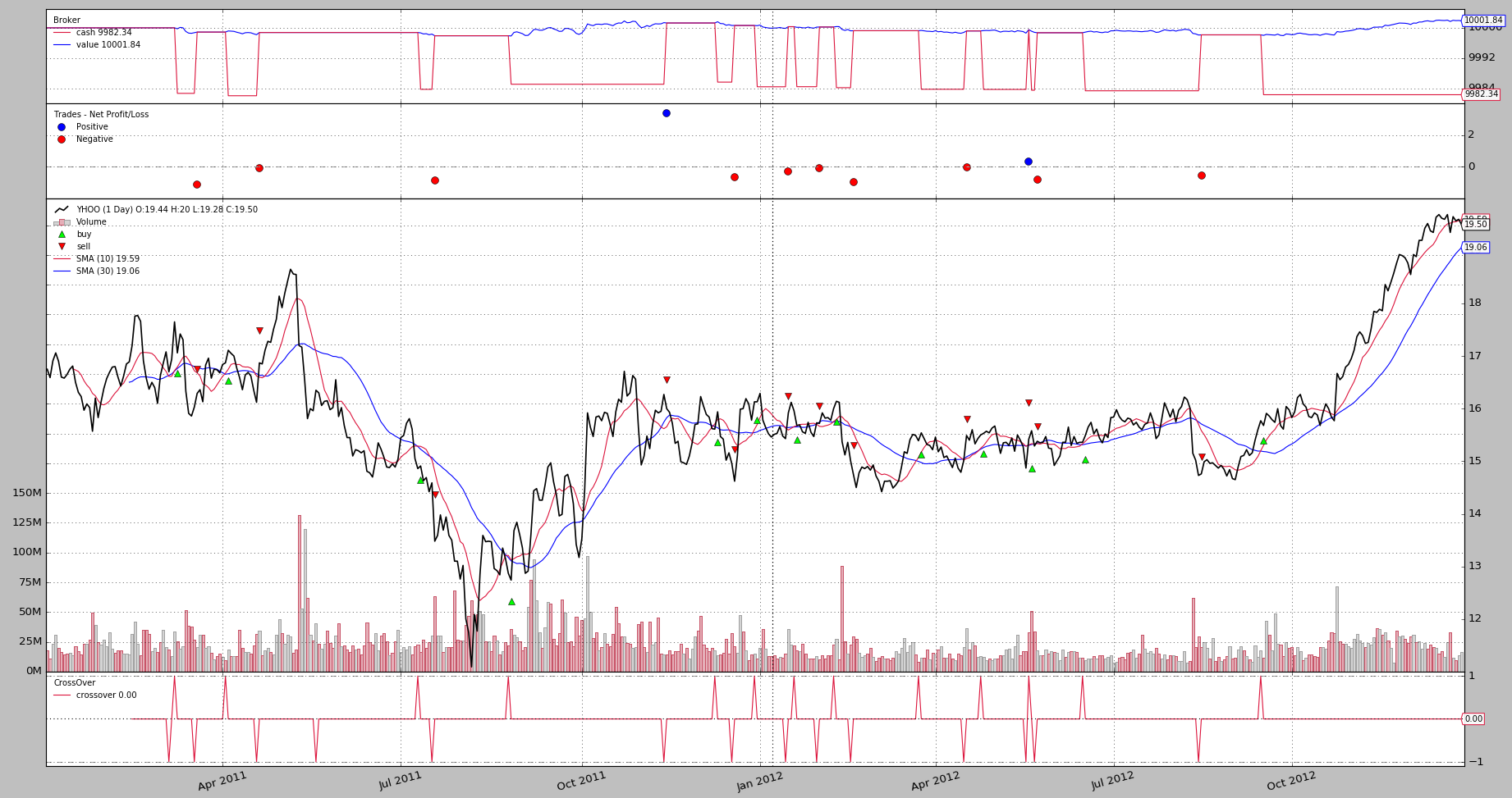
backtrader

from datetime import datetime
import backtrader as bt
    
class SmaCross(bt.SignalStrategy):
    def __init__(self):
        sma1, sma2 = bt.ind.SMA(period=10), bt.ind.SMA(period=30)
        crossover = bt.ind.CrossOver(sma1, sma2)
        self.signal_add(bt.SIGNAL_LONG, crossover)
    
cerebro = bt.Cerebro()
cerebro.addstrategy(SmaCross)
    
data0 = bt.feeds.YahooFinanceData(dataname='YHOO', fromdate=datetime(2011, 1, 1),
                                  todate=datetime(2012, 12, 31))
cerebro.adddata(data0)
   
cerebro.run()
cerebro.plot()

Other

This is a python algorithmic trading library found elsewhere. ultra-finance QSTK