[PYTHON] An overview of DELG, a new method for extracting image features that attracts attention with Kaggle
Introduction
This article introduces the image feature extraction algorithm DELG, which is attracting attention in Google Landmark Recognition.
This algorithm was announced in January 2020, and it seems that there is almost no Japanese literature.
Overview
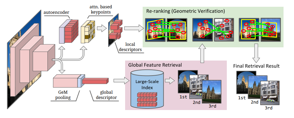
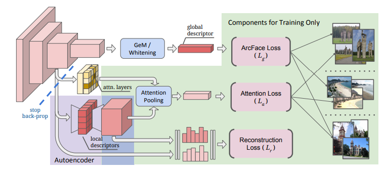
Image feature extraction is roughly divided into Global feature that reflects the information of the entire image and Local feature that collects local features. So far, different algorithms have been adopted for these two feature extractions. In this paper, these are combined into one algorithm for the purpose of efficient feature extraction. Specifically, this is achieved by using the average pooling layer for the Global feature and the attentive selection for the Local feature. It also introduces dimensionality reduction of local features based on autoencoder.
As a result, this model has achieved State of the art performance on a number of datasets (including Google's published Landmark dataset).

What is Global feature / Local feature?
Global feature is a feature extracted from the entire image. A Local feature is a collection of features extracted from a part of an image.
| Global feature (global descriptor, embedding) |
Local feature | |
|---|---|---|
| Range of extraction target | -The entire | -local |
| dimension | - 画像につき1dimension | - 画像につき複数dimensionになりうる |
| Extraction procedure | -Calculate the whole at once | 1.Select the local area to extract(detector) 2.Extract features(descriptor) |
| Feature | -Lightweight calculation because it is one step -Since the output is one-dimensional per image, the amount of data can be suppressed. -Excellent recall |
-Relatively robust even if part of the image is hidden -Excellent precision |
| Typical method | -Color histogram - GeM pooling - ArcFace loss |
- SIFT - SURF - RANSAC - DELF |
reference
- Combining Local and Global Image Features for Object Class Recognition -Large-scale image based on hashing of local features
You can see that the strengths and weaknesses of the Global feature and Local feature are different. Similar image selection algorithms (Retrival) generally have a two-step stance in which selection is performed by the Global feature and then geometric verification is performed by the local feature.
What is Autoencoder?
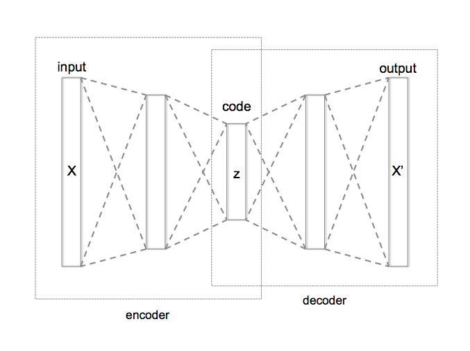
It is a dimension reduction method using a neural network, and the dimension is reduced by sandwiching an intermediate layer with a smaller number of nodes than the input layer.
Since Local features generally have a large dimension (100 to 1,000), it is customary to perform dimension reduction such as PCA separately. However, in this paper, we aim to reduce this dimension as a one-stop service, so we are using an Autoencoder that can be incorporated into a neural network to reduce the dimension.
Proposed model
The features of the proposed model are as follows. --Based on ResNet
- Global feature extraction --Adjusted output by Generalized mean average (GeM) and whitening of fully connected layer --Learning with ArcFace loss
- Local feature --The algorithm that distinguishes the characteristic locality is important. Adopt Attention module --Dimension reduction with autoencoder --Learning with attention loss and reconstruction loss

Implementation
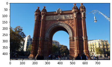
Extract the global feature and local feature of the following image.

Global feature
import tensorflow as tf

#Load the trained DELG model
SAVED_MODEL_DIR = '../input/delg-saved-models/local_and_global'
DELG_MODEL = tf.saved_model.load(SAVED_MODEL_DIR)

#Set parameters

##Dimension of Global feature to extract
NUM_EMBEDDING_DIMENSIONS = 2048
##Set the image resolution(Image Pyramids)
DELG_IMAGE_SCALES_TENSOR = tf.convert_to_tensor([0.70710677, 1.0, 1.4142135])
##Cut out only the part of the DELG model used for global feature extraction
DELG_INPUT_TENSOR_NAMES = ['input_image:0', 'input_scales:0']
GLOBAL_FEATURE_EXTRACTION_FN = DELG_MODEL.prune(DELG_INPUT_TENSOR_NAMES,
                                                ['global_descriptors:0'])


#Read image data as a tensor from the image path
# image_Please set the path appropriately
image_tensor = load_image_tensor(image_path)

#Extract Global feature with DELF
embedding_tensor_1 = GLOBAL_FEATURE_EXTRACTION_FN(image_tensor, DELG_IMAGE_SCALES_TENSOR)[0]

#Standardize
embedding_tensor_2 = tf.nn.l2_normalize(
    embedding_tensor_1,
    axis=1,
    name='l2_normalization')

#Combine results with different resolutions
embedding_tensor_3 = tf.reduce_sum(
    embedding_tensor_2, axis=0, name='sum_pooling')

#Further standardize this
embedding_res = tf.nn.l2_normalize(
    embedding_tensor_3, axis=0, name='final_l2_normalization').numpy()
| operation | size | |
|---|---|---|
| image_tensor | image data | 450, 800, 3 |
| embedding_tensor_1 | 2048 dimensional Global feature extraction for 3 resolutions | 3, 2048 |
| embedding_tensor_2 | Standardization | 3, 2048 |
| embedding_tensor_3 | Total in the direction of crushing the resolution axis | 2048, |
| embedding_res | Standardization | 2048, |
Local feature
#Set parameters
##Maximum number of features to be extracted
LOCAL_FEATURE_NUM_TENSOR = tf.constant(1000)

#Cut out the model
LOCAL_FEATURE_EXTRACTION_FN = DELG_MODEL.prune(
    DELG_INPUT_TENSOR_NAMES + ['input_max_feature_num:0', 'input_abs_thres:0'],
    ['boxes:0', 'features:0'])

#Load the image with a tensor
image_tensor = load_image_tensor(image_path)

#Extraction of local features by DELF
#Outputs the position and value of features
features = LOCAL_FEATURE_EXTRACTION_FN(image_tensor, DELG_IMAGE_SCALES_TENSOR,
                                       LOCAL_FEATURE_NUM_TENSOR,
                                       DELG_SCORE_THRESHOLD_TENSOR,
                                      )

#Position of the image extracted as a feature
#Add the 0th and 2nd columns, 1st and 3rd columns of the output and divide by 2.
keypoints = tf.divide(
  tf.add(
      tf.gather(features[0], [0, 1], axis=1),
      tf.gather(features[0], [2, 3], axis=1)), 2.0).numpy()


#Feature value
#Standardize
descriptors = tf.nn.l2_normalize(
  features[1], axis=1, name='l2_normalization').numpy()
train_keypoints = keypoints
train_descriptors = descriptors
test_keypoints = keypoints_2 #Comparison
test_descriptors = descriptors_2 #Comparison

#Convert descriptors to a tree structure and get points that are close in distance.
#Reference: https://myenigma.hatenablog.com/entry/2020/06/14/205753#kdtree%E3%81%A8%E3%81%AF
train_descriptor_tree = spatial.cKDTree(train_descriptors)
_, matches = train_descriptor_tree.query(
  test_descriptors, distance_upper_bound=max_distance)

test_kp_count = test_keypoints.shape[0]
train_kp_count = train_keypoints.shape[0]

test_matching_keypoints = np.array([
test_keypoints[i,]
  for i in range(test_kp_count)
 #Nearest neighbor point is max_If the distance is exceeded, the maximum index +1 will be returned.
  if matches[i] != train_kp_count
])
train_matching_keypoints = np.array([
  train_keypoints[matches[i],]
  for i in range(test_kp_count)
  if matches[i] != train_kp_count
])
The results of finding the local features of the two images to be compared and visualizing the matching parts based on the corresponding descriptors are shown below. It's a pity that the position doesn't fit exactly, but you can see that the characteristic parts are roughly associated.
| The original image | Data augmentation |
|---|---|
 |
 |
 |
 |
Field of development
With this, the local features and their countermeasures have been sought, but in more development, there are the following issues.
- I want to improve the accuracy of the corresponding points
- I want to understand the spatial relationship (understanding how different the images were taken, etc.)
The RANSAC algorithm is commonly used for these problems. Also, pydegensac is introduced in kaggle as a faster algorithm than RANSAC. The following articles are easy to understand, so please take a look.
reference: -Association of feature points by calculating "movement amount" and "deformation amount" of each image
At the end
See below for more details. -Original paper -Original implementation -Kernel used as reference for implementation
Recommended Posts
