From robots to self-driving cars to games such as Go and Shogi, many "AI" are becoming popular these days.

One of the keywords is "reinforcement learning". In that sense, it may be the most noticeable (and exaggerated ...) method of all machine learning methods.

This time, about the method of reinforcement learning, Deep Q-learning (so-called dokyun, DQN, which has recently achieved remarkable accuracy from the basics. )), I would like to explain the flow and mechanism of its development.

** A hands-on event was held based on the contents of this article (enhanced and revised version of [Talk of PyConJP) **

Reinforcement learning starting with Python OpenAI Gym experience hands-on

Lecture materials are richer in illustrations, so this is recommended for mathematical formulas and other things.

Characteristics of reinforcement learning

Reinforcement learning is similar to supervised learning, but it does not provide a clear "answer" (by the teacher). So what is presented is "action options" and "rewards."

If you think of this as the answer = reward, you may feel that it is the same (action A = 10pt, etc.), but there is one big difference. That is, the reward in reinforcement learning is not given to "each action", but to "the result of continuous actions". In soccer, one point for a goal is a reward for reinforcement learning. However, no reward is given for each action of passing or dribbling to reach the goal. On the other hand, supervised learning is when instructions are sent from outside the court, saying, "The current pass is good!" And "You shouldn't dribble there!" In reinforcement learning, only one goal as a "result of continuous action" is rewarded, so how good the pass and dribble to reach it is from the case where the goal was achieved and the case where it was not possible. You need to do the "evaluation" yourself.

So how do you "evaluate" each action? First, the action (last shot) at the moment of goal will be rewarded (1 point). But what about the action just before that? This was also the final setting for scoring a goal, so I think it was a pretty good move. Then, if you calculate back from the previous action, you can evaluate each action retroactively from the last action.

In reinforcement learning, the "evaluation" of each action is updated by oneself from the reward for the "result of continuous actions" in this way. In this way, even if you do not set a reward for each action one by one, you will learn continuous actions that will finally get a reward based on your own evaluation. In complex games such as shogi and go, it can be difficult to decide which move is best in which situation, let alone how many points the reward should be. Even in such a case, the final win or loss is clear, so by applying reinforcement learning, it is possible to skip the difficulty of behavior evaluation and learn the behavior to win in the end. As a result, reinforcement learning can handle more complex problems in general than supervised learning.

However, keep in mind that reinforcement learning is not a better method than supervised learning in this regard. Conversely, reinforcement learning takes a lot of time because it requires you to acquire an "evaluation of behavior" within yourself without clear instructions. The number of actions to reach the goal, and the number of combinations thereof, is enormous, and optimization takes a lot of time (although computers are computationally fast). In addition, there is no rational guarantee from the human point of view that the "evaluation of behavior" acquired by reinforcement learning is. It is clear that the former is more efficient and easier to reach the optimal solution if you have a proper teacher and if you study by yourself, so you need to choose the learning method appropriately according to the problem you are dealing with.

The above are the characteristics of reinforcement learning. Next, I will model this and explain how to learn it.

Modeling Reinforcement Learning (Markov Decision Process)

The problem targeted by reinforcement learning is modeled as follows.

States: S
Status. In the game, it represents a specific aspect
Model: T(s, a, s') (=P(s'|s, a))
T is Transition, and if action a is taken in situation s, it becomes situation s'. However, it is a probabilistic expression (P (s'| s, a)) because it expresses a situation where even if a is selected, it does not activate or goes to another place.
Actions: A(s), A
Action. If the action that can be taken changes depending on the situation, it becomes a function such as A (s).
Reward: R(s), R(s, a), R(s, a , s')
Situations and rewards from actions in those situations. This reward is self-assessed except for the final result (immediate reward).
Policy: \pi(s) -> a
Strategy. A function that returns what action a should be taken in the situation s.

This modeling is called the Markov Decision Process (MDP, Markov decision process). Markov means Markov property, which means that only the current state (s) is involved in the next action as represented by $ \ pi (s) $.

To explain it as a street fighter, it looks like the following.

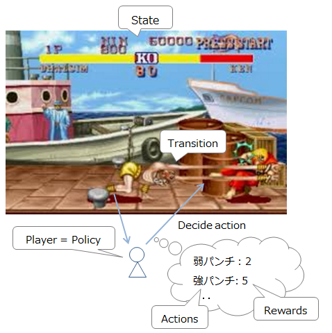
Current situation (enemy / own position and HP): State
Currently available commands: Actions
Movement / attack etc: T (s, a, s') List of commands that can be entered and their activation probabilities (because you may make a mistake in the command even if you try to issue a yoga fire, it becomes probabilistic)
Player (decision maker): Policy
Action rewards: Reward
In addition, I received a comment that "I wanted you to make the strongest strike 2 warrior by machine learning", but the fighting ability of AI has already exceeded that of ordinary people, and on the contrary, "how to adjust" is an issue. (Reference). Mankind needs to work hard at training.

By the way, in street fighting, shaving the opponent's HP is the shortest path to win, but it is clear that it is difficult to win in the end even with just punching. Therefore, in order to optimize the strategy, it is necessary to maximize the reward in the long term, not in the short term.

However, if the time is infinite even for a long period of time, zoom punching (see the figure above) is the most efficient strategy as far as possible. This is because if you have infinite time, it is safer to take measures to at least keep away from your opponent than to risk approaching and doing yoga flames. In this way, when the time is infinite, we tend to be biased toward low-risk, low-return behavior, so we will introduce the concept of time discount. In other words, if you don't act quickly, the rewards you get for the same action will decrease steadily.

In other words, the following two points are important for optimizing the strategy.

Try to optimize the sum of rewards
Introduce reward discounts over time

This can be expressed as an expression as follows.

U^{\pi}(s) = E \left[ \sum_{t}^{\infty} \gamma^{t} R(s_t) | \pi, s_0=s \right]

Sum of rewards = $ U ^ {\ pi} (s) $: Sum of rewards when performing strategy $ \ pi $ from state $ s $ ($ \ pi, s_0 = s $)
Discount on time = $ \ gamma $: $ 0 \ leq \ gamma <1 $, a value close to 1

The goal is to discover a strategy that maximizes this "sum of rewards considering time discounts". Let's call this optimal strategy $ \ pi ^ * $. In the best strategy, you should basically act to maximize your reward. This can be expressed mathematically as follows.

\pi^{*}(s) = argmax_a \sum_{s'} T(s, a, s') U(s')

$ argmax $ means pick the largest one. In other words, out of $ s'$, which is the transition destination from $ s $, the total expected reward $ U (s') $ acts toward the maximum $ s'$. After all, the optimal strategy $ \ pi ^ * $ is to act in such a way that the sum of the rewards from any $ s $ is maximized, so $ U ^ {\ defined at the beginning. You can rewrite pi} (s) $ as follows:

U(s) = R(s) + \gamma max \sum_{s'} T(s, a, s') U(s')

This equation is called ** Bellman equation **. The reason I rewrote it this way is that I was able to get the strategy $ \ pi $ out of the formula so that I could "calculate its reward regardless of the strategy I chose." In other words, the optimal behavior can be calculated only from the game settings (environment). This is the key item for training the model.

Model learning

From here, I will explain how to train the model built above.

Value Iteration

Using the Bellman equation derived earlier, let's calculate the optimal behavior "from the environment only". In this calculation, as explained in the first section, the calculation is repeated from the state where the "last reward" was obtained. This iterative calculation is called ** Value Iteration **.

Below, the state of Value Iteration is illustrated using the example of Pac-Man.

It is modeled after Markov Decision Processes and Reinforcement Learning, p18 ~ 21.

If you write down this situation, it will be as follows.

Set a fixed reward
For each state s, calculate the reward obtained by viable a

\gamma \sum T(s, a, s') U(s')

Calculate the total reward $ U (s) $ at a, which gives the highest reward in 1.

U(s) = R(s) + \gamma max \sum_{s'} T(s, a, s') U(s') = Bellman Equation!

Return to 1 until it converges (until the update width of $ U (s) $ becomes smaller) and repeat the update.

It has been proven that it will eventually converge to the expected value.

In this way, Value Iteration was able to estimate the reward map "from the environment only". However, in this state, all actions that can be placed in all situations are thoroughly investigated, so the optimum action can be derived, but it is not very efficient. Therefore, first decide on an appropriate strategy, then search for rewards within that range and consider a method of updating. That is Policy Iteration.

Policy Iteration

In Policy Iteration, first decide on a suitable (random) strategy $ \ pi_0 $. Then you can calculate the "reward from the strategy" $ U ^ {\ pi_0} (s) , and improve the strategy based on it ( \ pi_1 $). In other words, the steps are as follows.

Decide on an appropriate strategy ($ \ pi_0 $)
Calculate $ U ^ {\ pi_t} (s) $ based on your strategy
Update strategy $ \ pi_t $ to $ \ pi_ {t + 1} . ( \ pi_ {t + 1} = argmax_a \ sum T (s, a, s') U ^ {\ pi_t} (s') $)
Return to 1 until it converges and repeat the update

Convergence means $ \ pi_ {t + 1} \ approx \ pi_ {t} $, that is, when the selected behavior is almost unchanged. This iteration is called ** Policy Iteration **.

Now, it seems that the optimal strategy can be calculated by Value Iteration and Policy Iteration. However, as you can see from the formula, this calculation requires that $ T (s, a, s') $ be known. In other words, it is necessary to clarify in advance the transition destination when acting in each situation. This is a delicately large constraint, and especially when there are a large number of situations and actions that can be taken, it is very difficult to set everything like "This is what happens here ...".

Q-learning, which will be introduced in the next section, solves this problem. It is also called "Model-Free" learning method because it does not require prior environment (model) settings.

Q-learning

Then, how do you learn in Q-learning without information on the environment (model)? The answer is "try it first". Even if $ T (s, a, s') $ is unknown, if you take action a in the state s once, s'will become clear, so you will learn by repeating this "trial". .. Of course, it takes a lot of time to do such a thing, so in that sense there is an advantage that it is not necessary to set the model in advance, but on the other hand, it is a handicap in terms of learning time.

The formula for "try it first" is as follows.

Q(s, a) \approx R(s, a) + \gamma max_{a'} E[Q(s', a')]

$ T (s, a, s') $ has disappeared and is now the expected value ($ E [Q (s', a')] ). This expected value will be refined by repeating the trial. Therefore, in the end, the expressions that are almost equal ( \ approx ) above will be established as equations. Because, the fact that the equation holds means that the expected value ( Q (s, a) ) and the expected value when actually acting ( R (s, a) + \ gamma max_ {a'} E [ This is because Q (s', a')] $) is equal, which means that we have an accurate estimate of the reward. This is a guide for completing learning.

The formula for this learning process is as follows.

Q(s, a) = Q(s, a) + \alpha(\underline{R(s, a) + \gamma max_{a'} E[Q(s', a')]} - \underline{Q(s, a)})

$ \ Alpha $ is the learning rate, which means that you will learn from the difference between the expected value ($ \ approx $ actual reward) and the expected value. This difference (= error) is called TD error (TD = Temporal Difference), and the method of learning based on TD error is called TD learning. In other words, Q-learning is a kind of TD learning.

The above formula is also applied as follows.

Q(s, a) = (1 - \alpha)\underline{Q(s, a)} + \alpha(\underline{R(s, a) + \gamma max_{a'} E[Q(s', a')]})

It's getting a little complicated, but in the end, it's trying to clarify "what kind of state, how to act, and what kind of reward". This reward forecast table is called the Q-Table (see figure below).

Markov Decision Processes and Reinforcement Learning, p39

From p39 to p46 of the above material, you can check how the Q-Table is updated, that is, how the learning progresses, so please refer to it (0.9 in the material is $). \ gamma $, the discount rate of the reward).

Now we can improve $ Q (s, a) $ more and more ... but there is still the question of how to decide a in the first place. In short, you should choose the one with the largest $ Q (s, a) $, but if you do this, you will continue to select the "maximum known", so the reward is still unknown. It will destroy the chances of getting to the high $ s'$. Take an unknown path where there may be treasure, or a stable path with known rewards ... This is a trade-off and is called an exploitation and exploitation dilemma. I will.

There are several approaches to this problem, but the basic method is the ε-greedy method. It is a method of adventuring with a probability of ε, and then greedy, that is, acting based on a known reward. Another Boltzmann distribution ($ P (a | s) = \ frac {e ^ {\ frac {Q (s, a)} {k}}} {\ sum_j e ^ {\ frac {Q (s, a_j)) There is a method using} {k}}} $), which is random when $ k $ is large, and becomes more rewarding while knowing as it becomes smaller.

It has been proved that if you repeat the action based on the strategy and update $ Q (s, a) $, it will eventually converge to the optimum value. Yes, someday ... However, since it is human beings who cannot wait someday, various attempts have been made to find out how to approximate the optimum $ Q (s, a) $. Among them, approximation using neural networks has led to DQN and Deep Q-learning, which have achieved remarkable accuracy in recent years.

Deep Q-learning

The basis of learning a neural network is the error propagation method (Back Propagation). In short, it is a method of adjusting the model so that it is close to the correct answer by calculating the error from the correct answer and propagating it in the opposite direction.

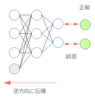Neural network starting with Chainer

Therefore, when approximating $ Q (s, a) $ with a neural network, the question is what is the "error"? Here, the error called "TD error" came out above.

Q(s, a) = Q(s, a) + \alpha(R(s, a) + \gamma max_{a'} E[Q(s', a')] - Q(s, a))

This was the difference between the expected value of the reward ($ \ approx $ actual reward) and the expected value. This is likely to be the starting point for the definition of error. First, neural net $ Q (s, a) $. The weight of the neural network at this time is $ \ theta $, and $ Q_ \ theta (s, a) $. Then, the definition of the error using the TD error in the above formula is multiplied as follows.

L_\theta = E[\frac{1}{2} (\underline{R(s, a) + \gamma max_{a'} Q_{\theta_{i-1}}(s', a')} - Q_\theta(s, a))^2]

The square is due to the error, and the $ \ frac {1} {2} $ is to eliminate the 2 that appears when differentiating ($ f (x) = x ^ 2 $). When $ f'(x) = 2x $). As you can see from the structure of the formula, the underlined part (expected value) is the teacher label (target) in supervised learning. Then, the gradient at the time of error propagation obtained by differentiating this equation is as follows.

\nabla_\theta L(\theta_i) = E[(\underline{R(s, a) + \gamma max Q_{\theta_{i-1}}(s', a')} - Q_{\theta_i}(s, a))\nabla_\theta Q_{\theta_i}(s, a)]

Now you are ready to go. However, who has a good understanding? You might think, but $ Q $ on the expected value side is $ Q_ {\ theta_ {i-1}} (s', a') $. This is because the expected value is calculated using the previous $ \ theta $. As mentioned above, this serves as a teacher label in supervised learning, so $ \ theta $ is included in the formula on the expected value side, but it is not a derivative when calculating the gradient. This point needs to be kept in mind when implementing.

Now, all I have to do is learn ... but in reality, learning as it is does not work very well. It's only natural that the parameters have increased due to the neural network. Therefore, some ingenuity in learning has been devised, and Deep Q-learning is possible only when this is included.

Experience Replay

The data given in reinforcement learning is, of course, continuous in chronological order. If this is the case, there will be a correlation between the data, so the goal of Experience Replay is to somehow break it apart.

The method is to first store the experienced state / behavior / reward / transition destination in the memory, and then randomly sample and use it when learning.

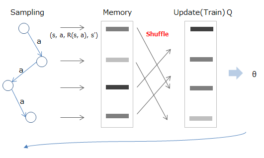
Mathematically, it is like sampling from the value stored in the memory (D) as shown below (red part) and learning using the calculated expected value (blue part).

Deep Reinforcement Learning/David Silver, Google DeepMind, p12

Fixed Target Q-Network

$ Q_ {\ theta_ {i-1}} (s', a') $ included in the expected value, which is the previous weight $ \ theta_ {i, even though it acts as a teacher label. It depends on -1} $. Therefore, the label will change as B, and $ \ theta $ are updated, although it was A before. It's a state of change in the morning.

Therefore, as in Experience Replay above, first extract some samples from the data to create a mini-batch, and during the learning, the $ \ theta $ used to calculate the expected value is fixed.

Mathematically, by fixing $ w ^-$ (red) used to calculate the expected value as shown below, the expected value (blue part) is stabilized. After learning is finished, update $ w ^-$ to $ w $ and move on to the calculation of the next batch.

Deep Reinforcement Learning/David Silver, Google DeepMind, p13

Reward clipping

This means that the reward to be given is fixed, so if it is positive, it will be 1 and if it is negative, it will be -1. Therefore, it is not possible to weight the reward (such as 10pt! Because I was able to reach the goal quickly), but at the cost of making learning easier.

As described above, Deep Q-learning includes the method of approximating Q-learning with a neural network and (at least) the above three techniques for efficient learning in that case. Neural network approximation also has the advantage that a numerical vector can now be received as the input for state s. In games such as breakout, this makes it possible to perform tricks such as vectorizing the game screen as it is and inputting and learning, and AlphaGo also uses the same method (using the image of the board as input as it is). ..

Deep Q-learning is currently undergoing various improvements, but I think that understanding the above contents will help you to understand when following the research trends.

Practice

Up to this point, the content was theoretical, so let's try it from here. There is a platform called Open AI that summarizes various learning environments for reinforcement learning. This time, I will use this to actually learn the algorithm.

OpenAI Gym OpenAI opens "training gym for AI"

As you can see here, various learning environments such as games are provided. It's fun just looking at it.

OpenAI Gym environments

This is actually a Python library, and the installation method is described in detail on the official GitHub.

openai/gym

The installation is basically pip install gym, but this can be run only in the following environment with the minimum configuration installation.

algorithmic
toy_text
classic_control (requires pyglet for drawing)

Other learning environments require additional installation. For example, if you want to run Atari games, you need to install additional modules with pip install gym [atari]. You may need to install something other than Python, so it's safe to include the one described in Installing everything. When using with Python3, please note the description of Supported-systems.

The usage is as described in Document, but it looks like the following.

import gym


env = gym.make('CartPole-v0')  # make your environment!

for i_episode in range(20):
    observation = env.reset()
    for t in range(100):
        env.render()  # render game screen
        action = env.action_space.sample()  # this is random action. replace here to your algorithm!
        observation, reward, done, info = env.step(action)  # get reward and next scene
        if done:
            print("Episode finished after {} timesteps".format(t+1))
            break

Initialize the environment with ʻenv.reset ()` (equivalent to resetting the game)
From the observed state (state = ʻobservation`), determine the action by some algorithm
Get the reward for the action and the next state transitioned by the action by'env.step (action)'
done indicates the end of the episode (with the result of the game). When you reach this point, go back to 1 and start learning again.

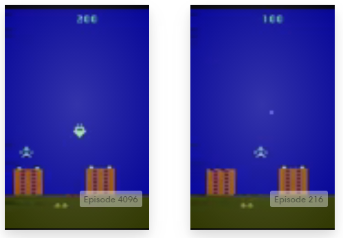
With ʻenv.monitor`, you can easily monitor accuracy and take videos. This result can also be uploaded to the OpenAI site, so if you're a kid, give it a try.

Here is the code that I actually implemented. Since the results are uploaded to OpenAI Gym, you can also check the evaluation results there (icoxfog417's algorithm).

icoxfog417/chainer_pong

When implementing, I referred to the following code.

It takes a lot of time to learn, so it takes a lot of time to determine if it's working (the gist code above takes about 3 days to learn). As with image recognition, in short, development is difficult without a GPU. In that sense, GPUs are becoming essential in modern machine learning if it's not just about running samples.

However, it is becoming easier to prepare an environment such as an AWS GPU instance, so please give it a try (although it will be very exciting when you launch an instance).

That is all for the explanation. I hope you can dive from zero to deep!

[PYTHON] Reinforcement learning to learn from zero to deep

Characteristics of reinforcement learning

Modeling Reinforcement Learning (Markov Decision Process)

Model learning

Reward clipping

Practice

References