[PYTHON] Complementing kaggle's titanic missing values and creating features
Introduction
Last time, I looked at Titanic's train data to see what features are related to survival rate. Last time: Data analysis before kaggle's titanic feature generation (I hope you can read this article as well)
Based on the result, this time ** we will create a data frame to complement the missing values and add the necessary features to give to the prediction model **.
This time, as a prediction model, we will use "** GBDT (gradient boosting tree) xg boost **", which is often used in kaggle competitions, so we will make the data suitable for it.
1. Data acquisition and missing value confirmation
import pandas as pd
import numpy as np

train = pd.read_csv('/kaggle/input/titanic/train.csv')
test = pd.read_csv('/kaggle/input/titanic/test.csv')
#Combine train data and test data into one
data = pd.concat([train,test]).reset_index(drop=True)
#Check the number of rows that contain missing values
train.isnull().sum()
test.isnull().sum()
The number of each missing value is as follows.
| train data | test data | |
|---|---|---|
| PassengerId | 0 | 0 |
| Survived | 0 | |
| Pclass | 0 | 0 |
| Name | 0 | 0 |
| Sex | 0 | 0 |
| Age | 177 | 86 |
| SibSp | 0 | 0 |
| Parch | 0 | 0 |
| Ticket | 0 | 0 |
| Fare | 0 | 1 |
| Cabin | 687 | 327 |
| Embarked | 2 | 0 |
2. Complement of Embarked and Fare
First, looking at the two rows where Embarked is missing, both ** Pclass is 1 ** and ** Fare is 80 **.
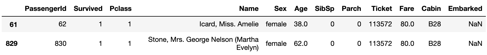 Among those with a'P class of 1'and a'Fare of 70-90', ** Embarked had the highest proportion of S **, so these two are complemented by S.
data['Embarked'] = data['Embarked'].fillna('S')
Next, regarding Fare, the ** P class of the missing line was 3 ** and ** Embarked was S **.
 Therefore, it is complemented by the median among those who meet these two conditions.
data['Fare'] = data['Fare'].fillna(data.query('Pclass==3 & Embarked=="S"')['Fare'].median())
Regarding the missing value of Age, I would like to ** predict the age using a random forest ** after creating other features, so I will describe it later.
3. Classification of features
** Family_size, Fare, Cabin, Ticket ** that combine Sibsp and Parch will be ** classified according to the difference in survival rate **. For the difference in survival rate for each feature, see the article Previous.
** Classification of feature quantity'Family_size' representing the number of family members **
data['Family_size'] = data['SibSp']+data['Parch']+1

data['Family_size_bin'] = 0
data.loc[(data['Family_size']>=2) & (data['Family_size']<=4),'Family_size_bin'] = 1
data.loc[(data['Family_size']>=5) & (data['Family_size']<=7),'Family_size_bin'] = 2
data.loc[(data['Family_size']>=8),'Family_size_bin'] = 3
** Fare classification **
data['Fare_bin'] = 0
data.loc[(data['Fare']>=10) & (data['Fare']<50), 'Fare_bin'] = 1
data.loc[(data['Fare']>=50) & (data['Fare']<100), 'Fare_bin'] = 2
data.loc[(data['Fare']>=100), 'Fare_bin'] = 3
** Cabin classification **
#Features representing the first alphabet'Cabin_label'Create(Missing value'n')
data['Cabin_label'] = data['Cabin'].map(lambda x:str(x)[0])

data['Cabin_label_bin'] = 0
data.loc[(data['Cabin_label']=='A')|(data['Cabin_label']=='G'), 'Cabin_label_bin'] = 1
data.loc[(data['Cabin_label']=='C')|(data['Cabin_label']=='F'), 'Cabin_label_bin'] = 2
data.loc[(data['Cabin_label']=='T'), 'Cabin_label_bin'] = 3
data.loc[(data['Cabin_label']=='n'), 'Cabin_label_bin'] = 4
** Classification by the number of duplicate Ticket numbers'Ticket_count'**
data['Ticket_count'] = data.groupby('Ticket')['PassengerId'].transform('count')

data['Ticket_count_bin'] = 0
data.loc[(data['Ticket_count']>=2) & (data['Ticket_count']<=4), 'Ticket_count_bin'] = 1
data.loc[(data['Ticket_count']>=5), 'Ticket_count_bin'] = 2
** Classification by Ticket number type **
#Divide into tickets with numbers only and tickets with numbers and alphabets
#Get a number-only ticket
num_ticket = data[data['Ticket'].str.match('[0-9]+')].copy()
num_ticket_index = num_ticket.index.values.tolist()
#Tickets with only numbers dropped from the original data and the rest contains alphabets
num_alpha_ticket = data.drop(num_ticket_index).copy()

#Classification of tickets with numbers only
#Since the ticket number is a character string, it is converted to a numerical value
num_ticket['Ticket'] = num_ticket['Ticket'].apply(lambda x:int(x))

num_ticket['Ticket_bin'] = 0
num_ticket.loc[(num_ticket['Ticket']>=100000) & (num_ticket['Ticket']<200000),
               'Ticket_bin'] = 1
num_ticket.loc[(num_ticket['Ticket']>=200000) & (num_ticket['Ticket']<300000),
               'Ticket_bin'] = 2
num_ticket.loc[(num_ticket['Ticket']>=300000),'Ticket_bin'] = 3

#Classification of tickets including numbers and alphabets
num_alpha_ticket['Ticket_bin'] = 4
num_alpha_ticket.loc[num_alpha_ticket['Ticket'].str.match('A.+'),'Ticket_bin'] = 5
num_alpha_ticket.loc[num_alpha_ticket['Ticket'].str.match('C.+'),'Ticket_bin'] = 6
num_alpha_ticket.loc[num_alpha_ticket['Ticket'].str.match('C\.*A\.*.+'),'Ticket_bin'] = 7
num_alpha_ticket.loc[num_alpha_ticket['Ticket'].str.match('F\.C.+'),'Ticket_bin'] = 8
num_alpha_ticket.loc[num_alpha_ticket['Ticket'].str.match('PC.+'),'Ticket_bin'] = 9
num_alpha_ticket.loc[num_alpha_ticket['Ticket'].str.match('S\.+.+'),'Ticket_bin'] = 10
num_alpha_ticket.loc[num_alpha_ticket['Ticket'].str.match('SC.+'),'Ticket_bin'] = 11
num_alpha_ticket.loc[num_alpha_ticket['Ticket'].str.match('SOTON.+'),'Ticket_bin'] = 12
num_alpha_ticket.loc[num_alpha_ticket['Ticket'].str.match('STON.+'),'Ticket_bin'] = 13
num_alpha_ticket.loc[num_alpha_ticket['Ticket'].str.match('W\.*/C.+'),'Ticket_bin'] = 14

data = pd.concat([num_ticket,num_alpha_ticket]).sort_values('PassengerId')
4. Age complement
For the missing value of Age, there is a method of ** median ** or ** finding and complementing the average age for each title of the name **, but when I looked it up, it was lost using a random forest. There was a method ** to predict the age of the part where it is, so this time I will use that.
from sklearn.preprocessing import LabelEncoder
from sklearn.ensemble import RandomForestRegressor
#Label non-numerical features numerically
#Also label features that are not used to predict Age
le = LabelEncoder()
data['Sex'] = le.fit_transform(data['Sex'])
data['Embarked'] = le.fit_transform(data['Embarked'])
data['Cabin_label'] = le.fit_transform(data['Cabin_label'])

#Features used to predict Age'age_data'Put in
age_data = data[['Age','Pclass','Family_size',
                 'Fare_bin','Cabin_label','Ticket_count']].copy()
#Divide into missing and non-missing rows
known_age = age_data[age_data['Age'].notnull()].values
unknown_age = age_data[age_data['Age'].isnull()].values

x = known_age[:, 1:]
y = known_age[:, 0]
#Learn in Random Forest
rfr = RandomForestRegressor(random_state=0, n_estimators=100, n_jobs=-1)
rfr.fit(x, y)
#Predict the value and assign it to the missing row
age_predict = rfr.predict(unknown_age[:, 1:])
data.loc[(data['Age'].isnull()), 'Age'] = np.round(age_predict,1)
You have now completed the missing value for Age.
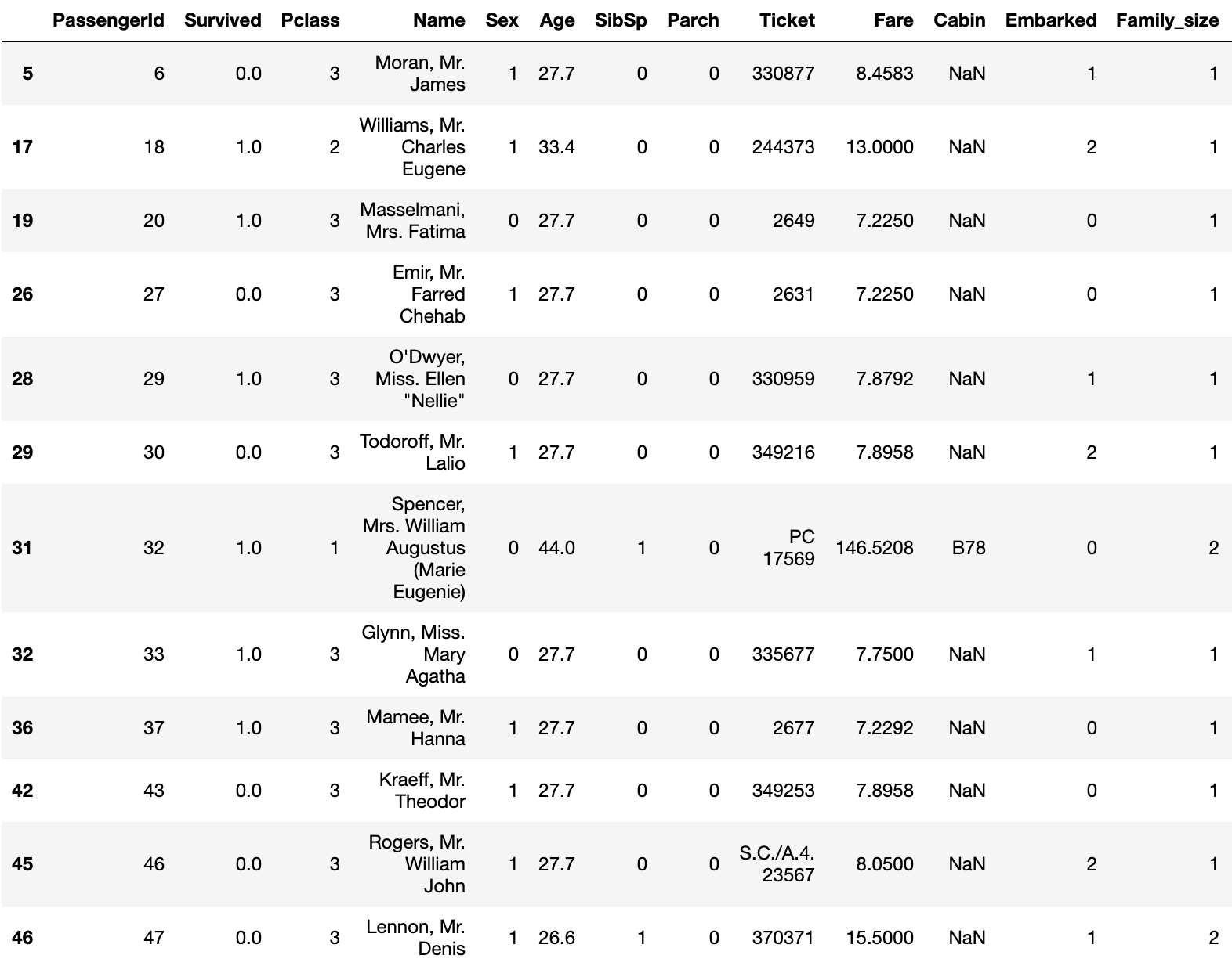 And Age will also be classified.
data['Age_bin'] = 0
data.loc[(data['Age']>10) & (data['Age']<=30),'Age_bin'] = 1
data.loc[(data['Age']>30) & (data['Age']<=50),'Age_bin'] = 2
data.loc[(data['Age']>50) & (data['Age']<=70),'Age_bin'] = 3
data.loc[(data['Age']>70),'Age_bin'] = 4
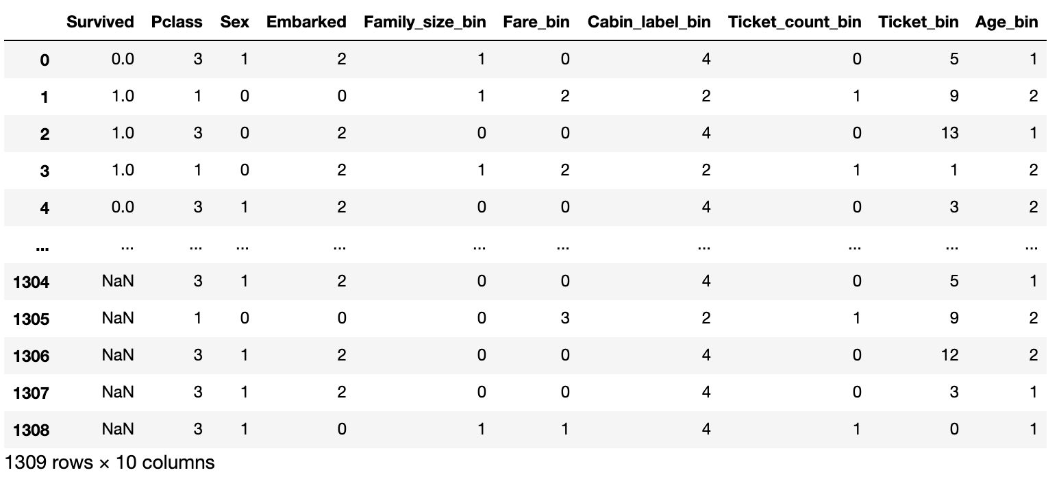
At the end, the unnecessary features are dropped and the feature creation is completed.
#Remove unnecessary features.
data = data.drop(['PassengerId','Name','Age','Fare','SibSp','Parch','Ticket','Cabin',
                  'Family_size','Cabin_label','Ticket_count'], axis=1)
In the end, the dataframe looks like this.
5. Forecast with xg boost
First, the data is divided into train data and test data again, and it is divided into'X'only for features and'Y' for only'Survived'.
#Divide into train data and test data again
model_train = data[:891]
model_test = data[891:]

X = model_train.drop('Survived', axis=1)
Y = pd.DataFrame(model_train['Survived'])
x_test = model_test.drop('Survived', axis=1)
Let's look at the performance of the model by seeking two, ** logloss ** and ** accuracy **.
from sklearn.metrics import log_loss
from sklearn.metrics import accuracy_score
from sklearn.model_selection import KFold
import xgboost as xgb
#Set parameters
params = {'objective':'binary:logistic',
          'max_depth':5,
          'eta': 0.1,
          'min_child_weight':1.0,
          'gamma':0.0,
          'colsample_bytree':0.8,
          'subsample':0.8}

num_round = 1000

logloss = []
accuracy = []

kf = KFold(n_splits=4, shuffle=True, random_state=0)
for train_index, valid_index in kf.split(X):
    x_train, x_valid = X.iloc[train_index], X.iloc[valid_index]
    y_train, y_valid = Y.iloc[train_index], Y.iloc[valid_index]
    #Convert data frame to a shape suitable for xg boost
    dtrain = xgb.DMatrix(x_train, label=y_train)
    dvalid = xgb.DMatrix(x_valid, label=y_valid)
    dtest = xgb.DMatrix(x_test)
    #Learn with xgboost
    model = xgb.train(params, dtrain, num_round,evals=[(dtrain,'train'),(dvalid,'eval')],
                      early_stopping_rounds=50)

    valid_pred_proba = model.predict(dvalid)
    #Ask for log loss
    score = log_loss(y_valid, valid_pred_proba)
    logloss.append(score)
    #Find accuracy
    #valid_pred_Since proba is a probability value, it is converted to 0 and 1.
    valid_pred = np.where(valid_pred_proba >0.5,1,0)
    acc = accuracy_score(y_valid, valid_pred)
    accuracy.append(acc)

print(f'log_loss:{np.mean(logloss)}')
print(f'accuracy:{np.mean(accuracy)}')
With this code log_loss : 0.4234131996311837 accuracy : 0.8114369975356523 The result was that.
Now that we have a model, we will create forecast data to submit to kaggle.
y_pred_proba = model.predict(dtest)
y_pred= np.where(y_pred_proba > 0.5,1,0)

submission = pd.DataFrame({'PassengerId':test['PassengerId'], 'Survived':y_pred})
submission.to_csv('titanic_xgboost.csv', index=False)
The result looks like this.
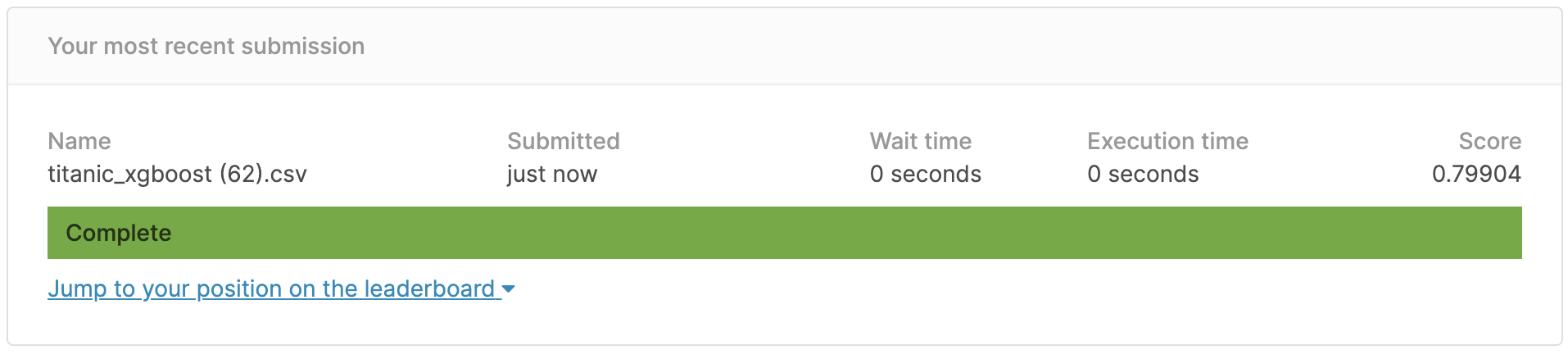 The correct answer rate was ** 79.9% **, which did not reach 80%, but it seems that it can reach 80% by adjusting the parameters of the model.
Summary
This time I tried to actually submit the predicted value to kaggle.
Cabin data that I thought could not be used as a feature because there were many missing values, but when I tried labeling each missing value, the accuracy rate of the predicted value increased **, and the feature amount that can be used if the data is properly processed. I found out that. Also, if you make predictions without classifying features such as Fare and Age, ** logloss and accuracy values will improve **, but ** the accuracy rate of the predicted values will not improve **. I felt that it would be possible to create an appropriate model without overfitting by classifying the features based on the difference in survival rate rather than using them as they are.
If you have any opinions or suggestions, we would appreciate it if you could make a comment or edit request.
Sites and books that I referred to
Kaggle Tutorial Titanic know-how to be in the top 2% pyhaya’s diary Book: [Kaggle Winning Data Analysis Technology](https://www.amazon.co.jp/Kaggle%E3%81%A7%E5%8B%9D%E3%81%A4%E3%83%87% E3% 83% BC% E3% 82% BF% E5% 88% 86% E6% 9E% 90% E3% 81% AE% E6% 8A% 80% E8% A1% 93-% E9% 96% 80% E8 % 84% 87-% E5% A4% A7% E8% BC% 94-ebook / dp / B07YTDBC3Z)