[PYTHON] Dimensionality reduction and 2D plotting techniques for high-dimensional data

Introduction

This article uses Python 2.7, numpy 1.11, scipy 0.17, scikit-learn 0.18, matplotlib 1.5, seaborn 0.7, pandas 0.17. It has been confirmed to work on jupyter notebook. (Please modify% matplotlib inline appropriately) I refer to the article of Manifold learning of Sklearn.

A technique called manifold learning will be explained using a sample sklearn digits. In particular, t-SNE is a method suitable for visualization of multidimensional data, which is sometimes used in Kaggle and the like. In addition to visualization, you can improve the accuracy of simple classification problems by combining the original data and the compressed data.

table of contents

1. Data generation
2. Dimensionality reduction focusing on linear elements
   1. Random Projection
   2. PCA
   3. Linear Discriminant Analysis
3. Dimensionality reduction considering non-linear components
   1. Isomap
   2. Locally Linear Embedding
   3. Modified Locally Linear Embedding
   4. Hessian Eigenmapping
   5. Spectral Embedding
   6. Local Tangent Space Alignment
   7. Multi-dimensional Scaling
   8. t-SNE
   9. Random Forest Embedding

1. Data generation

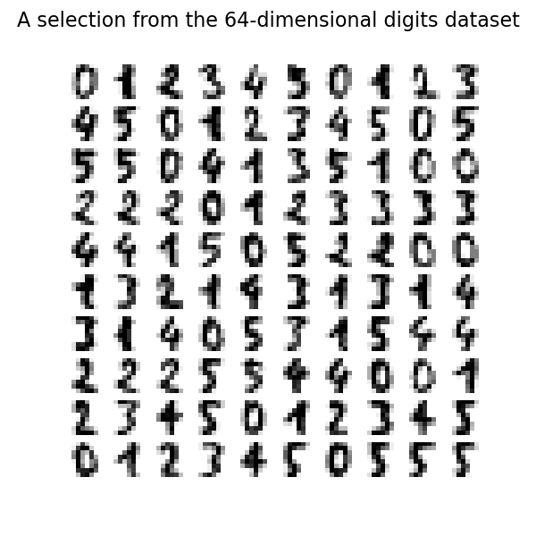
We will use the sample data of sklearn. This time, we will cluster the numbers using the digits dataset. First, load and check the data.

load_digit.py

from time import time

import numpy as np
import matplotlib.pyplot as plt
from matplotlib import offsetbox
from sklearn import (manifold, datasets, decomposition, ensemble,
                     discriminant_analysis, random_projection)

digits = datasets.load_digits(n_class=6)
X = digits.data
y = digits.target
n_samples, n_features = X.shape
n_neighbors = 30

n_img_per_row = 20
img = np.zeros((10 * n_img_per_row, 10 * n_img_per_row))
for i in range(n_img_per_row):
    ix = 10 * i + 1
    for j in range(n_img_per_row):
        iy = 10 * j + 1
        img[ix:ix + 8, iy:iy + 8] = X[i * n_img_per_row + j].reshape((8, 8))

plt.imshow(img, cmap=plt.cm.binary)
plt.xticks([])
plt.yticks([])
plt.title('A selection from the 64-dimensional digits dataset')

Prepare a function for mapping digit data. This is not the subject of this article, so skip it if you are not sure.

def plot_embedding(X, title=None):
    x_min, x_max = np.min(X, 0), np.max(X, 0)
    X = (X - x_min) / (x_max - x_min)

    plt.figure()
    ax = plt.subplot(111)
    for i in range(X.shape[0]):
        plt.text(X[i, 0], X[i, 1], str(digits.target[i]),
                 color=plt.cm.Set1(y[i] / 10.),
                 fontdict={'weight': 'bold', 'size': 9})

    if hasattr(offsetbox, 'AnnotationBbox'):
        # only print thumbnails with matplotlib > 1.0
        shown_images = np.array([[1., 1.]])  # just something big
        for i in range(digits.data.shape[0]):
            dist = np.sum((X[i] - shown_images) ** 2, 1)
            if np.min(dist) < 4e-3:
                # don't show points that are too close
                continue
            shown_images = np.r_[shown_images, [X[i]]]
            imagebox = offsetbox.AnnotationBbox(
                offsetbox.OffsetImage(digits.images[i], cmap=plt.cm.gray_r),
                X[i])
            ax.add_artist(imagebox)
    plt.xticks([]), plt.yticks([])
    if title is not None:
        plt.title(title)

2. Dimensionality reduction focusing on linear components

The method introduced here has low computational cost and high versatility, and is frequently used. For example, PCA is a very convenient method for extracting data correlation. These methods are explained in detail on many sites, so let's take a quick look.

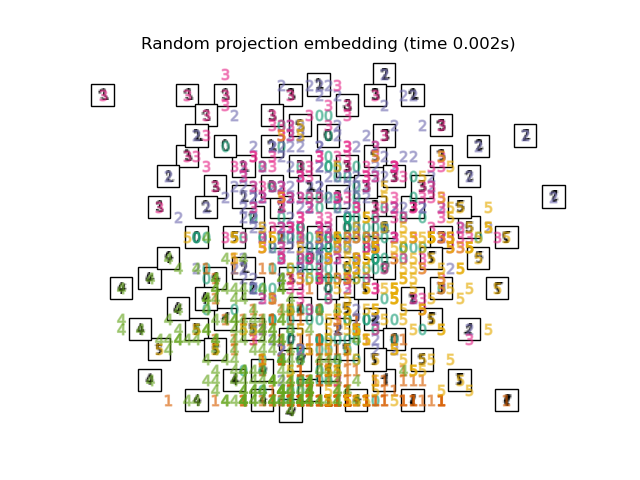
2.1. Random Projection I got 64 dimensional numerical data in 1. The most basic method for mapping such high-dimensional data is Random Projection. Using a very simple method, the elements of the matrix R that maps M-dimensional data to mappable N-dimensional are set with random numbers. The merit is the low calculation cost.

print("Computing random projection")
rp = random_projection.SparseRandomProjection(n_components=2, random_state=42)
X_projected = rp.fit_transform(X)
plot_embedding(X_projected, "Random Projection of the digits")
#plt.scatter(X_projected[:, 0], X_projected[:, 1])

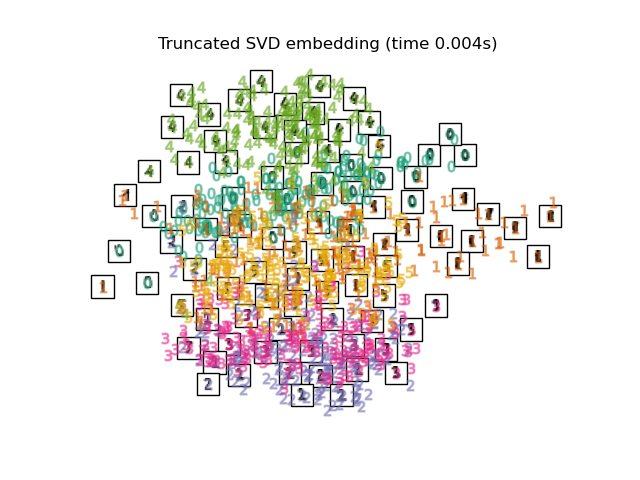
2.2. PCA Map with PCA, which is a general dimensional compression method. Extract the correlation component between variables. The function used is sklearn's Truncated SVD, and the difference from PCA seems to be whether to normalize the input data.

print("Computing PCA projection")
t0 = time()
X_pca = decomposition.TruncatedSVD(n_components=2).fit_transform(X)
plot_embedding(X_pca,
               "Principal Components projection of the digits (time %.2fs)" %
               (time() - t0))

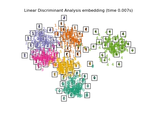
2.3. Linear Discriminant Analysis Dimensionality reduction is performed by Linear discriminant analysis. The Mahalanobis distance is used on the assumption that each variable has a multivariate normal distribution and the same group has the same covariance matrix. Similar to PCA, but this is supervised learning.

print("Computing Linear Discriminant Analysis projection")
X2 = X.copy()
X2.flat[::X.shape[1] + 1] += 0.01  # Make X invertible
t0 = time()
X_lda = discriminant_analysis.LinearDiscriminantAnalysis(n_components=2).fit_transform(X2, y)
plot_embedding(X_lda,
               "Linear Discriminant projection of the digits (time %.2fs)" %
               (time() - t0))

3. Dimensionality reduction considering non-linear components

The three methods introduced earlier are not suitable in terms of dimensionality reduction of data with a hierarchical structure and data containing non-linear components. Here we introduce a two-dimensional plot of non-linearly correlated data, such as swiss roll.

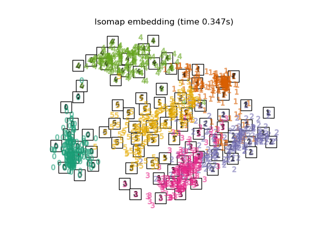
3.1. Isomap Isomap is one of the dimension reduction / clustering methods considering non-linearity. Calculate the geodesic distance along the shape of the manifold and perform Multi-Dimensional Scaling based on it. It can be executed with Sklearn's Isomap function. BallTree is used at the stage of calculating the measured distance.

print("Computing Isomap embedding")
t0 = time()
X_iso = manifold.Isomap(n_neighbors, n_components=2).fit_transform(X)
print("Done.")
plot_embedding(X_iso,
               "Isomap projection of the digits (time %.2fs)" %
               (time() - t0))

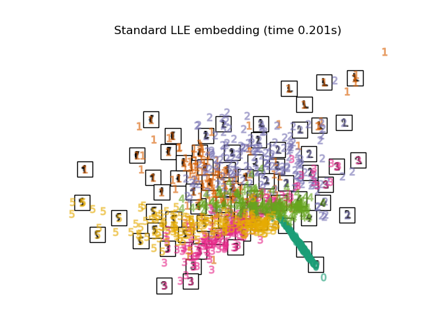
3.2. Locally Linear Embedding (LLE) Even a manifold that includes non-linearity as a whole. A dimension reduction method based on the intuition of linearity when viewed locally. The 0 label appears to be emphasized, but the other labels are messed up.

print("Computing LLE embedding")
clf = manifold.LocallyLinearEmbedding(n_neighbors, n_components=2,
                                      method='standard')
t0 = time()
X_lle = clf.fit_transform(X)
print("Done. Reconstruction error: %g" % clf.reconstruction_error_)
plot_embedding(X_lle,
               "Locally Linear Embedding of the digits (time %.2fs)" %
               (time() - t0))

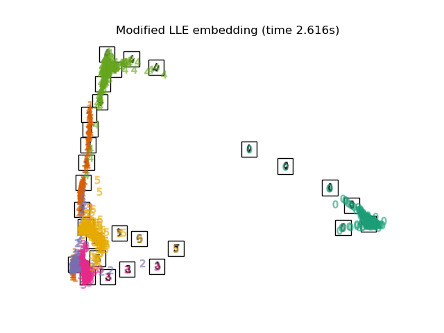
3.3. Modified Locally Linear Embedding An algorithm that improves the regularization problem, which has the problem of LLE. 0 Labels are clearly classified. The 4, 1, 5 labels also look nicely mapped.

print("Computing modified LLE embedding")
clf = manifold.LocallyLinearEmbedding(n_neighbors, n_components=2,
                                      method='modified')
t0 = time()
X_mlle = clf.fit_transform(X)
print("Done. Reconstruction error: %g" % clf.reconstruction_error_)
plot_embedding(X_mlle,
               "Modified Locally Linear Embedding of the digits (time %.2fs)" %
               (time() - t0))

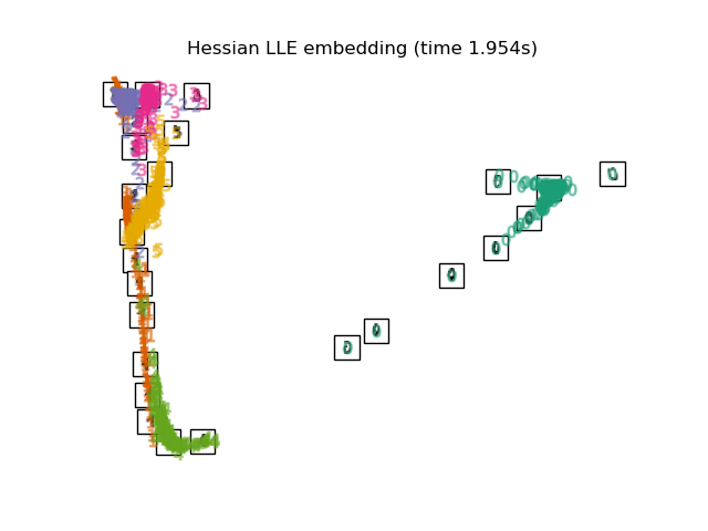
3.4. Hessian LLE Embedding An algorithm that improves the regularization problem, which has the problem of LLE. Part 2

print("Computing Hessian LLE embedding")
clf = manifold.LocallyLinearEmbedding(n_neighbors, n_components=2,
                                      method='hessian')
t0 = time()
X_hlle = clf.fit_transform(X)
print("Done. Reconstruction error: %g" % clf.reconstruction_error_)
plot_embedding(X_hlle,
               "Hessian Locally Linear Embedding of the digits (time %.2fs)" %
               (time() - t0))

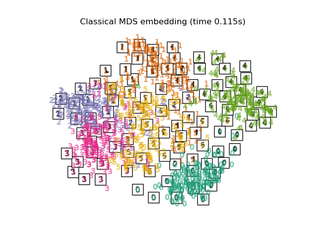
3.5. Spectral Embedding It is a compression method also called Laplacian Eigenmaps. I haven't investigated the technical content, but it seems that I am using the spectral graph theory. The shape of the mapping is different from LLE, MLLE, HLLE, but the distance and density between the label groups seem to be similar.

print("Computing Spectral embedding")
embedder = manifold.SpectralEmbedding(n_components=2, random_state=0,
                                      eigen_solver="arpack")
t0 = time()
X_se = embedder.fit_transform(X)

plot_embedding(X_se,
               "Spectral embedding of the digits (time %.2fs)" %
               (time() - t0))

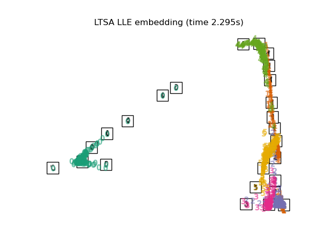
3.6. Local Tangent Space Alignment

The result is like reversing MLLE and HLLE. The classification results are similar.

print("Computing LTSA embedding")
clf = manifold.LocallyLinearEmbedding(n_neighbors, n_components=2,
                                      method='ltsa')
t0 = time()
X_ltsa = clf.fit_transform(X)
print("Done. Reconstruction error: %g" % clf.reconstruction_error_)
plot_embedding(X_ltsa,
               "Local Tangent Space Alignment of the digits (time %.2fs)" %
               (time() - t0))

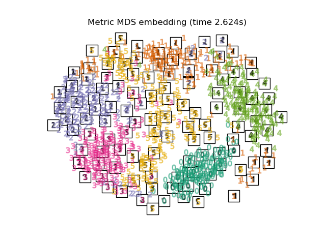
3.7. Multi-dimensional Scaling (MDS) [Multidimensional Scaling](https://ja.wikipedia.org/wiki/%E5%A4%9A%E6%AC%A1%E5%85%83%E5%B0%BA%E5%BA%A6 It is a compression method called% E6% A7% 8B% E6% 88% 90% E6% B3% 95). MDS itself seems to be a general term that summarizes several methods, but the details are not specifically summarized.

print("Computing MDS embedding")
clf = manifold.MDS(n_components=2, n_init=1, max_iter=100)
t0 = time()
X_mds = clf.fit_transform(X)
print("Done. Stress: %f" % clf.stress_)
plot_embedding(X_mds,
               "MDS embedding of the digits (time %.2fs)" %
               (time() - t0))

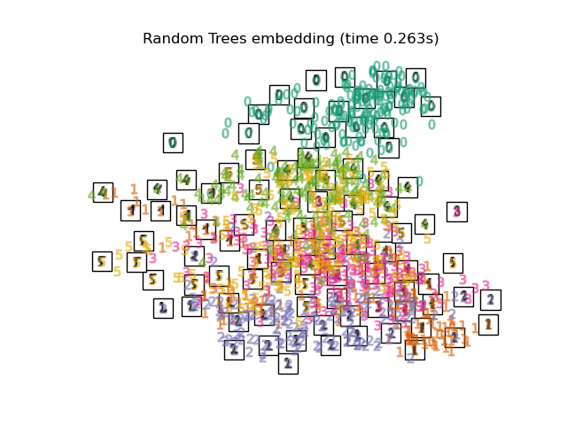
3.8. t-distributed Stochastic Neighbor Embedding (t-SNE) It is a method to convert the Euclidean distance of each point into a conditional probability instead of the similarity and map it to a lower dimension.

There is also a method called Barnes-Hut t-SNE, which improves the calculation cost at the expense of accuracy. In Sklearn, you can select two methods, exact (precision-oriented) and Barnes-Hut. By default, Barnes-Hut is selected, and tuning is possible by setting the optional angle as well. It's also frequently featured on Kaggle.

print("Computing t-SNE embedding")
tsne = manifold.TSNE(n_components=2, init='pca', random_state=0)
t0 = time()
X_tsne = tsne.fit_transform(X)

plot_embedding(X_tsne,
               "t-SNE embedding of the digits (time %.2fs)" %
               (time() - t0))

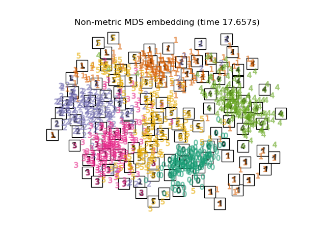
3.9. Random Forest Embedding

print("Computing Totally Random Trees embedding")
hasher = ensemble.RandomTreesEmbedding(n_estimators=200, random_state=0,
                                       max_depth=5)
t0 = time()
X_transformed = hasher.fit_transform(X)
pca = decomposition.TruncatedSVD(n_components=2)
X_reduced = pca.fit_transform(X_transformed)

plot_embedding(X_reduced,
               "Random forest embedding of the digits (time %.2fs)" %
               (time() - t0))