[PYTHON] Predict the distribution of continuous values other than the normal distribution with ordinary PyTorch or TensorFlow
Introduction
The other day, when I was looking at the implementation of muzero-general, there was an interesting way to categorically predict continuous values.
If you think about it carefully, I thought that it would be possible to express the prediction of an arbitrary probability distribution of continuous values, and when I verified it, it seemed to work, so I'll make a note of it.
Predict continuous values categorically
If you use MeanSquaredError to predict continuous values, you basically assume that the distribution of the values you want to predict is a normal distribution (and you are only interested in the expected values). So, for example, if the distribution has two mountains, it may be a little inconvenient to predict the distance between them. I don't know how wide it is (dispersion, etc.). If you have a fixed range of values (of interest), you can do the following:
For example, if the range of values is 0 to 10, then you decide on a point with a value of 11 such as v = [0, 1, 2, ..., 10].
First, set p [0 ~ 10] = 0,
For example, the value 3.7 is expressed as p [3] = 0.3, p [4] = 0.7. If it is 0.1, then p [0] = 0.9 and p [1] = 0.1. If it is 3, p [3] = 1.0. In short, it feels like allocating the degree of belonging to both ends of the value.
Conversely, if you want to calculate the original value from this p, calculate the expected value sum (p * v).
If you write it in code, it will look like this.
import numpy as np

SUPPORT_SIZE = 11
VALUE_RANGE = [0., 10.]


def scalar_to_support(scalars):
  values = np.array(scalars)
  min_v, max_v = VALUE_RANGE
  values = np.clip((values - min_v) / (max_v - min_v), 0., 1.)
  key_values = np.linspace(0., 1., SUPPORT_SIZE)

  r_index = np.searchsorted(key_values, values, side="left")  # a[i-1] < x <= a[i]
  l_index = np.clip(r_index-1, 0, len(key_values))
  left_vs = key_values[l_index]
  right_vs = key_values[r_index]

  interval = key_values[1] - key_values[0]
  left_ps = 1-(values - left_vs)/interval
  right_ps = 1-(right_vs - values)/interval

  vectors = np.zeros((len(values), SUPPORT_SIZE))
  for i in range(len(scalars)):
    vectors[i, l_index[i]] = left_ps[i]
    vectors[i, r_index[i]] = right_ps[i]

  return vectors

def support_to_scalar(supports):
  min_v, max_v = VALUE_RANGE
  key_values = np.linspace(min_v, max_v, SUPPORT_SIZE)
  supports /= supports.sum(axis=1, keepdims=True)
  return np.sum(supports * key_values, axis=1)
- In the implementation of muzero, an interesting conversion is performed as a pre-processing, but it is omitted.
For training, the output should be softmax (11 elements in this case) and the Loss function should be CrossEntropy.
Verification of whether the probability distribution can be learned
Let's verify it using the PyTorch that we just learned.
Prediction of constants
First, let's see if we can predict one value in a fixed manner.
code
# on jupyter notebook
import torch
import torch.nn.functional as F
import matplotlib.pyplot as plt

SUPPORT_SIZE = 101


class Net(torch.nn.Module):
  def __init__(self):
    super().__init__()
    self.fc = torch.nn.Linear(1, SUPPORT_SIZE)

  def forward(self, x):
    x = self.fc(x)
    x = F.softmax(x, dim=1)
    return x


def get_dummy_input(batch_size):
    dummy_inputs = np.random.random((batch_size, 1)).astype("float32")
    return torch.tensor(dummy_inputs)  # dummy

def constant_target_value_fn(const):
  def fn(batch_size):
    return [const] * batch_size
  return fn

def train_model(model, target_value_fn, epoch=1000, lr=0.01, batch_size=16):
  optimizer = torch.optim.Adam(model.parameters(), lr=lr)

  loss_history = []
  for ep in range(epoch):
    target_values = target_value_fn(batch_size)
    target_supports = torch.tensor(scalar_to_support(target_values))
    #
    optimizer.zero_grad()
    outputs = model(get_dummy_input(batch_size))
    losses = torch.mean(- target_supports * torch.log(outputs))
    losses.backward()
    optimizer.step()
    loss_history.append(losses.item())

  plt.plot(loss_history)
  plt.show()

#######################

model = Net()
train_model(model, constant_target_value_fn(4.8))
outputs = model(get_dummy_input(5)).detach().numpy()
print(f"Expected value={np.mean(support_to_scalar(outputs))}")

vs = np.mean(outputs, axis=0)
plt.plot(vs)
I set the target range to 0 to 10 and the size of the output vector to 101, and predicted a constant of 4.8. The prediction result is like this. There seems to be no problem.
Expected value = 4.840604254500373
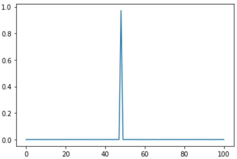
- The horizontal axis is 0 to 100, but please think that it is 0 to 10. The same applies thereafter.
Prediction of normal distribution
Next, let's train the normal distribution (loc = 4.8, scale = 0.9).
code
from scipy import stats

def norm_fn(loc, scale):
  def fn(batch_size):
    dist = stats.norm(loc=loc, scale=scale)
    return dist.rvs(batch_size)
  return fn

model = Net()
distribution_fn = norm_fn(4.8, 0.9)
train_model(model, distribution_fn, epoch=1000, batch_size=1024)
outputs = model(get_dummy_input(5)).detach().numpy()
print(f"Expected value={np.mean(support_to_scalar(outputs))}")

vs = np.mean(outputs, axis=0)
plt.plot(vs)
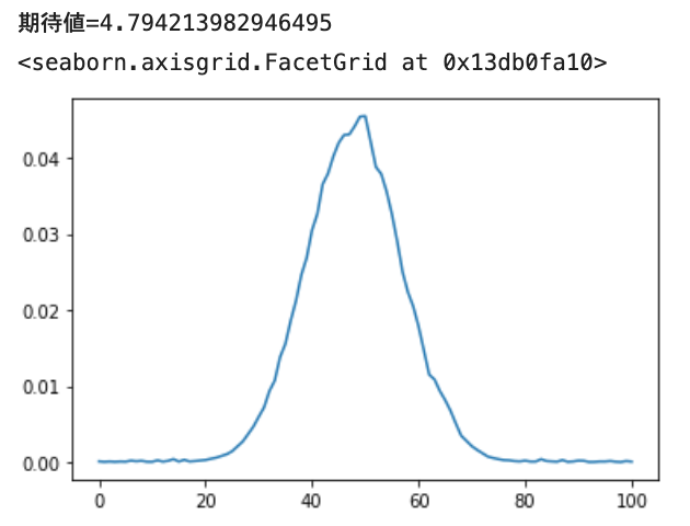
Good vibes.
Prediction of mixed normal distribution
Next, let's learn two normal distributions, Normal (loc = 1.8, scale = 0.3, probability = 0.6) and Normal (loc = 6.8, scale = 0.9, probability = 0.4).
code
from collections import Counter
def multi_norm_fn(loc_scale_prob_list):
  def fn(batch_size):
    values = []
    for loc, scale, prob in loc_scale_prob_list:
      dist = stats.norm(loc=loc, scale=scale)
      values.append(dist.rvs(batch_size))
    ps = np.array([p for _, _, p in loc_scale_prob_list])
    ps = ps / np.sum(ps)
    count = Counter(np.random.choice(range(len(values)), size=batch_size, p=ps))
    ret = []
    for i, cnt in count.items():
      ret += list(values[i][:cnt])
    return ret
  return fn


model = Net()
distribution_fn = multi_norm_fn([
  [1.8, 0.3, 0.6],
  [6.8, 0.9, 0.4],
])
train_model(model, distribution_fn, epoch=1000, batch_size=1024)
outputs = model(get_dummy_input(5)).detach().numpy()
print(f"Expected value={np.mean(support_to_scalar(outputs))}")

vs = np.mean(outputs, axis=0)
plt.plot(vs)
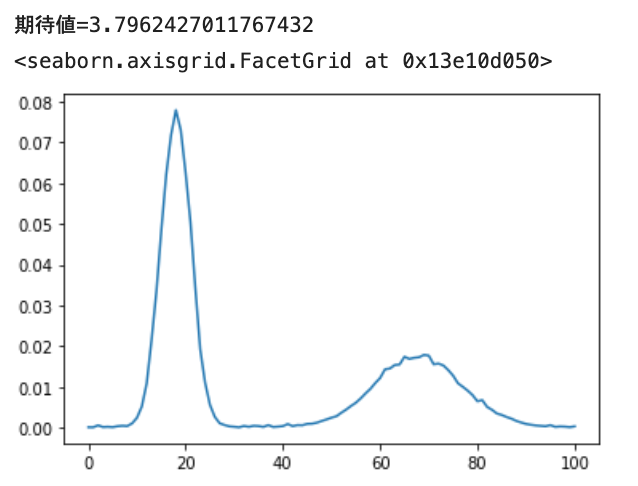
Oh, you can do two mountains properly. Also, the size of the base is expressed.
Exponential distribution prediction
Finally, there is the exponential distribution (loc = 1.4, scale = 2.0).
- The normal exponential distribution (2) is translated to the right by 1.4.
code
def exp_fn(loc, scale):
  def fn(batch_size):
    dist = stats.expon(loc, scale)
    return dist.rvs(batch_size)
  return fn

model = Net()
distribution_fn = exp_fn(1.4, 2.0)
train_model(model, distribution_fn, epoch=1000, batch_size=1024)
outputs = model(get_dummy_input(5)).detach().numpy()
print(f"Expected value={np.mean(support_to_scalar(outputs))}")

vs = np.mean(outputs, axis=0)
plt.plot(vs)
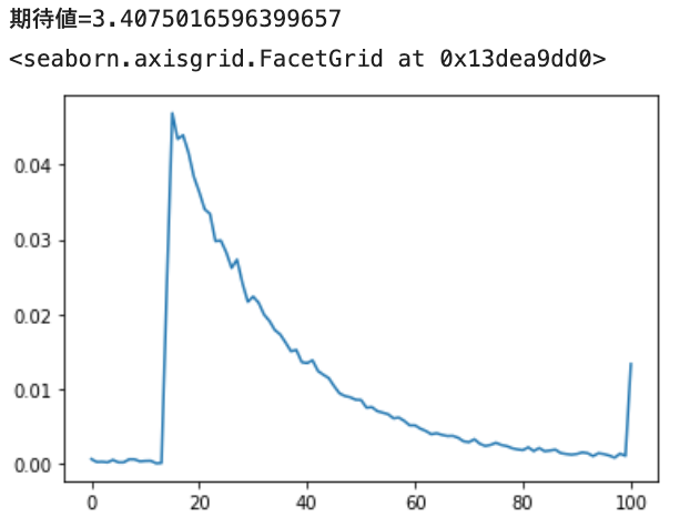
It is expressed that the peak rises from around 1.4 and gradually falls. It also shows that there are some values above 10.
Digression
Also, I think it's quite perfect for predicting continuous values that circulate like angles. It seems that 10 degrees and 350 degrees are actually close to each other with a little ingenuity.
at the end
So, I was able to confirm that continuous value prediction is OK with Cross Entropy in Categorical. This kind of technique may be mentioned in recent books, but I personally made a note of it because it was new.
Recommended Posts