[PYTHON] I was delighted to think that I was able to create a Holy Grail program that hits a rate prediction accuracy rate of 88% for FX (dollar yen) with deep learning, but when I predicted it with production data, it was a knack for repeating "I do not know".
About this article
I'm sorry for the article title like Naro. "With Deep Learning (CNN), make a dollar-yen forecasting program and be a millionaire!" As a result of enthusiasm, it is a story that failed __. __ On the other hand, please refer only to those who want to be a teacher __.
Description of the deliverable
I don't want to explain too much, but I will explain the deliverables.
Learn how to predict rates on a large number of chart images with CNN (Convolutional Neural Network)
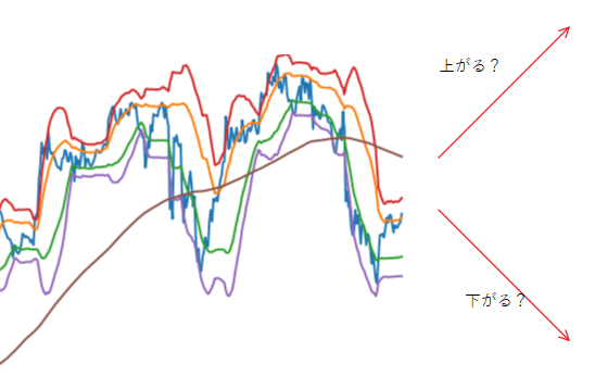
I created a program that outputs 3 choices of "up", "down", and "don't know" the rate after 24 hours.
 The inference result was a good result with a correct answer rate of 88%.
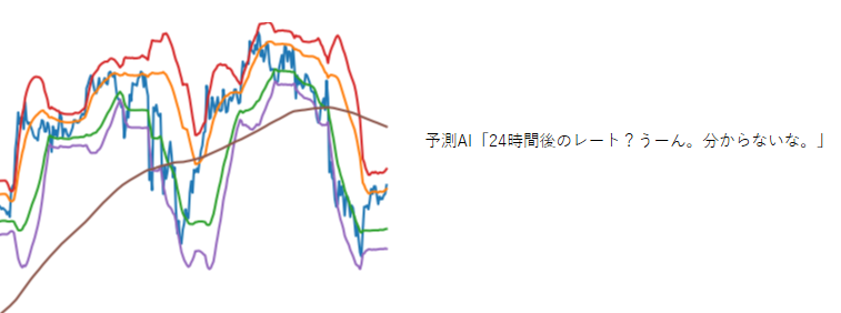
However, if you make a prediction based on actual data, you will get a lot of "I don't know". ..
It took 3 days to create it, so I'm not sure how it's done.
I learned a lot from the process of creating it, so I will leave it as an output.
The inference result was a good result with a correct answer rate of 88%.
However, if you make a prediction based on actual data, you will get a lot of "I don't know". ..
It took 3 days to create it, so I'm not sure how it's done.
I learned a lot from the process of creating it, so I will leave it as an output.
Construction environment
Built on Google Colaboratory. Python 3.6 Tensorflow 1.13.1
Data preprocessing
Image data preparation
CNN is deep learning of image classification.
Therefore, it is necessary to prepare a large number of chart images.
We prepared about 80,000 images as shown below.
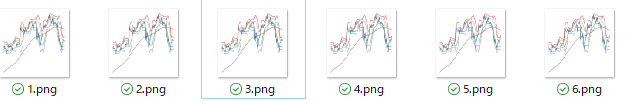 In addition, although it took about 8 hours to create 80,000 images, I actually used 30,000 for the reason described later.
Please refer to this article for how to create a chart image.
In addition, although it took about 8 hours to create 80,000 images, I actually used 30,000 for the reason described later.
Please refer to this article for how to create a chart image.
Arrangement of image data and storage in binary format
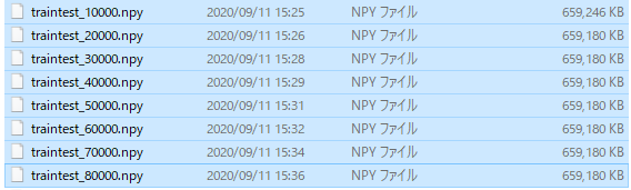
Learning work cannot be done with image data as it is. I need to convert the image data to a numpy array, and I saved it in npy format every 10,000 images.
import glob
import cv2
import numpy as np

X=[]

#List the target images
img_list = glob.glob('<Image save destination folder>/*.png')

#Resize image
for i in range(len(file_list)):
    file_name = '../Make_img/USDJPY/' + str(i) + '.png'
    img = cv2.imread(file_name)
    img = cv2.resize(img, dsize=(150, 150)) #resize
    X.append(img) #Add to list

    #Save every 10,000 sheets in binary format
    if (i > 0) and (i % 10000 == 0):
        #Convert to numpy and save binary
        X = np.array(X)
        npy_name = 'traintest_' + str(i) + '.npy'
        np.save(npy_name, X)
        X = []
Then, there are 0.7GB of npy files per one,
With 80,000 sheets, the capacity has become close to 6GB.
This time, the data saved on Google Drive, I plan to load it with Google Colob and work on it. It is not good to upload such a large file. Compress multiple npy files into one and combine them in npz format.
- I will realize later that it was not necessary to convert the array to npy and save it from the beginning.
arr1 = np.load('traintest_10000.npy')
arr2 = np.load('traintest_20000.npy')
arr3 = np.load('traintest_30000.npy')
arr4 = np.load('traintest_40000.npy')
arr5 = np.load('traintest_50000.npy')
arr6 = np.load('traintest_60000.npy')
arr7 = np.load('traintest_70000.npy')
arr8 = np.load('traintest_80000.npy')

np.savez_compressed('traintest_all.npz', arr1 , arr2, arr3, arr4, arr5, arr6, arr7, arr8)
When compressed, it became about 0.7GB.

Initially, I resized it to 250 * 250, As a result of loading with Google Colab, the memory crashed and I changed the size to 150 * 150. With this size, there are some parts that are blurred, and I'm worried whether I can grasp the features well. This may be one of the reasons why this prediction failed.
Read training data, test data, and correct labels with Google Colab
Upload the created npz file to Google Drive and Start GoogleColab and load it.
#Package import
from tensorflow.keras.callbacks import LearningRateScheduler
from tensorflow.keras.layers import Activation, Add, BatchNormalization, Conv2D, Dense, GlobalAveragePooling2D, Input
from tensorflow.keras.models import Model
from tensorflow.keras.optimizers import SGD
from tensorflow.keras.preprocessing.image import ImageDataGenerator
from tensorflow.keras.regularizers import l2
from tensorflow.keras.utils import to_categorical
import numpy as np
import matplotlib.pyplot as plt
import pandas as pd
%matplotlib inline
#Google Drive mount
from google.colab import drive
drive.mount('/content/drive')
#Read the npz that is the source of the dataset
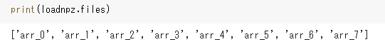
loadnpz = np.load(r'/content/drive/My Drive/traintest_all.npz')
Make sure that 8 items have been read properly.
Next, separate the images for training and verification. Read 10,000 sheets each.
- If you read more than this, the memory will crash during learning.
#Training and test image dataset
train_images = loadnpz['arr_0']
test_images = loadnpz['arr_1']
After reading the CSV file containing the correct answer label with DataFrame, it is converted to array. After conversion, separate the correct label for training and verification.
#Set of correct labels
df = pd.read_csv(r'/content/drive/My Drive/Colab Notebooks/npy file/tarintest_labels.csv')
df['target'] = df['target'].replace('Up', '0')
df['target'] = df['target'].replace('Down', '1')
df['target'] = df['target'].replace('Flat', '2')
df['target'] = df['target'].astype('int')
labels_arr = df['target'].to_numpy() #Convert label part to array

#Separate label data
train_labels = labels_arr[0:10001] #For training
test_labels = labels_arr[10001:20001] #For verification
Label data is converted to One Hot format.
#Convert to One Hot format
train_labels = to_categorical(train_labels)
test_labels = to_categorical(test_labels)
If you can do this, let's check the number of Shapes.
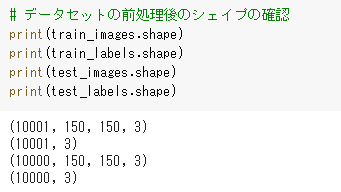
Modeling
Next is the creation of the model. This time, we will create it with a structure called ResNet. If you are wondering what ResNet is, please refer to this article .
If the image data to be read is too large, the memory will crash repeatedly and will not proceed at all. In that case, it is necessary to reduce batch_size during learning or reduce the image data itself. In my case, I initially used 250 * 250 image data and couldn't proceed all the way due to a series of memory crashes, so I resized it to 150 * 150.
#Generation of convolutional layer
def conv(filters, kernel_size, strides=1):
    return Conv2D(filters, kernel_size, strides=strides, padding='same', use_bias=False,
        kernel_initializer='he_normal', kernel_regularizer=l2(0.0001))

#Generation of residual block A
def first_residual_unit(filters, strides):
    def f(x):
        # →BN→ReLU
        x = BatchNormalization()(x)
        b = Activation('relu')(x)

        #Convolution layer → BN → ReLU
        x = conv(filters // 4, 1, strides)(b)
        x = BatchNormalization()(x)
        x = Activation('relu')(x)

        #Convolution layer → BN → ReLU
        x = conv(filters // 4, 3)(x)
        x = BatchNormalization()(x)
        x = Activation('relu')(x)

        #Convolution layer →
        x = conv(filters, 1)(x)

        #Adjust the shape size of the shortcut
        sc = conv(filters, 1, strides)(b)

        # Add
        return Add()([x, sc])
    return f

#Generation of residual block B
def residual_unit(filters):
    def f(x):
        sc = x

        # →BN→ReLU
        x = BatchNormalization()(x)
        x = Activation('relu')(x)

        #Convolution layer → BN → ReLU
        x = conv(filters // 4, 1)(x)
        x = BatchNormalization()(x)
        x = Activation('relu')(x)

        #Convolution layer → BN → ReLU
        x = conv(filters // 4, 3)(x)
        x = BatchNormalization()(x)
        x = Activation('relu')(x)

        #Convolution layer →
        x = conv(filters, 1)(x)

        # Add
        return Add()([x, sc])
    return f

#Generation of residual block A and residual block B x 17
def residual_block(filters, strides, unit_size):
    def f(x):
        x = first_residual_unit(filters, strides)(x)
        for i in range(unit_size-1):
            x = residual_unit(filters)(x)
        return x
    return f

#Input data shape
input = Input(shape=(150,150, 3))

#Convolution layer
x = conv(16, 3)(input)

#Residual block x 54
x = residual_block(64, 1, 18)(x)
x = residual_block(128, 2, 18)(x)
x = residual_block(256, 2, 18)(x)

# →BN→ReLU
x = BatchNormalization()(x)
x = Activation('relu')(x)

#Pooling layer
x = GlobalAveragePooling2D()(x)

#Fully connected layer
output = Dense(3, activation='softmax', kernel_regularizer=l2(0.0001))(x)

#Creating a model
model = Model(inputs=input, outputs=output)

#Conversion to TPU model
import tensorflow as tf
import os
tpu_model = tf.contrib.tpu.keras_to_tpu_model(
    model,
    strategy=tf.contrib.tpu.TPUDistributionStrategy(
        tf.contrib.cluster_resolver.TPUClusterResolver(tpu='grpc://' + os.environ['COLAB_TPU_ADDR'])
    )
)

#compile
tpu_model.compile(loss='categorical_crossentropy', optimizer=SGD(momentum=0.9), metrics=['acc'])

#ImageDataGenerator preparation
train_gen  = ImageDataGenerator(
    featurewise_center=True,
    featurewise_std_normalization=True)
test_gen = ImageDataGenerator(
    featurewise_center=True,
    featurewise_std_normalization=True)

#Pre-calculate statistics for the entire dataset
for data in (train_gen, test_gen):
    data.fit(train_images)
Learning
Carry out learning work. Even though I converted it to the TPU model, it takes nearly 5 hours because of the capacity.
#Preparing for LearningRateScheduler
def step_decay(epoch):
    x = 0.1
    if epoch >= 80: x = 0.01
    if epoch >= 120: x = 0.001
    return x
lr_decay = LearningRateScheduler(step_decay)

#Learning
batch_size = 32
history = tpu_model.fit_generator(
    train_gen.flow(train_images, train_labels, batch_size=batch_size),
    epochs=100,
    steps_per_epoch=train_images.shape[0] // batch_size,
    validation_data=test_gen.flow(test_images, test_labels, batch_size=batch_size),
    validation_steps=test_images.shape[0] // batch_size,
    callbacks=[lr_decay])
After learning, the correct answer rate (val_acc) in the verification data will be 88%!

Forecast with real data
Load new verification data into test_images and try to predict.
test_predictions = new_model.predict_generator(
    test_gen.flow(test_images[0:10000], shuffle = False, batch_size=16),
    steps=16)
test_predictions = np.argmax(test_predictions, axis=1)[0:10000]
The prediction result is output with 3 choices: "0: go up", "1: go down", and "2: don't know". Let's check.
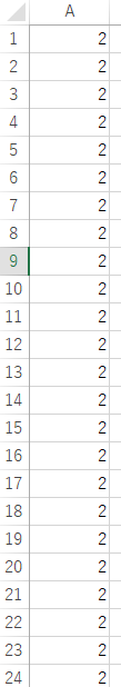
"2: I don't know" is repeated ... In some places, there were "0: go up" and "1: go down", The correct answer rate was a disastrous result of less than 50% ...
Why did you fail?
I think the following two are big.
- The image size after resizing was too small and the features were too rough.
- Too few images during the verification period
1 can be solved by increasing the size of the image, The free Google Colab environment is tough. If you become a paid member with a monthly fee of $ 10, it seems that you will be able to use twice as much memory, so it may be solved.
2 can improve to some extent because you can learn various chart patterns by shuffling all the images. It may also be possible to deliberately simplify the image itself and increase the number of similar charts. The Bollinger Bands are used in the article, but it may be improved by removing them and plotting only the closing price and the moving average.
Countermeasure 2 can be done for free, so I will try it in my spare time.