[PYTHON] Ford-Fulkerson Method and Its Applications-Supplement to Chapter 8 of the Algorithm Quick Reference-
Overview
This is a series of reading books, re-studying various things, and writing what you are interested in. This time, [Algorithm Quick Reference](http://www.amazon.co.jp/%E3%82%A2%E3%83%AB%E3%82%B4%E3%83%AA%E3%82% BA% E3% 83% A0% E3% 82% AF% E3% 82% A4% E3% 83% 83% E3% 82% AF% E3% 83% AA% E3% 83% 95% E3% 82% A1% E3% 83% AC% E3% 83% B3% E3% 82% B9-George-T-Heineman / dp / 4873114284) The theme is "Network Flow Algorithm" in Chapter 8. Overall, the Ford-Fulkerson method is amazing.
Main story 1: Outline of Ford-Fulkerson method
About various quantities on the graph
Edges on the (directed) graph are often weighted. The amount of this weight is
――Time and distance, --It's a cost --Some flow rate,
It corresponds to various concepts, but all are formulated as the same "edge weighting".
Dijkstra in Chapter 6 describes how to take this amount of weight as time and distance and perform calculations corresponding to "how long does it take to reach the goal point from a certain start point?" I am thinking by law. In this chapter, we will consider the costs and flow rates mentioned in the above example.
Ford-Fulkerson method and its points
First, consider flow rate = flow. There is a well-known method called the Ford-Fulkerson method. I think the idea of greedily increasing the number of ways to increase is relatively easy to understand, but I think the important point is to "think about the flow in the opposite direction to the normal direction." Here, I will try to explain with an emphasis on that idea.
For the sake of clarity, consider the graph in the following figure, which has a weight of 1 on each side, and find the maximum flow from S to T in this graph.
 In this graph, there are the following three routes from S to T, and all routes are exhausted only by this route.

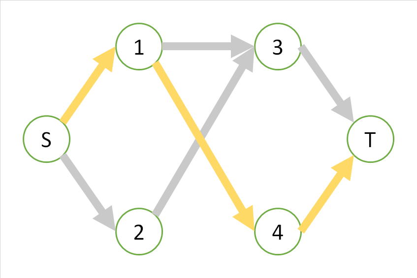
 For the time being, looking at the first orange route, this route cannot be used at the same time as the yellow or blue route. In that sense, if you take one orange path, you will not be able to increase the flow any more "by adding more parallel paths to the orange path", and the flow seems to be "maximum". ..
On the other hand, since the yellow path and the blue path can be taken at the same time, even if only the yellow path or the blue path is taken, they are not "maximum", and the path that takes yellow and blue at the same time is "maximum". There seems to be. And in this case, it is also the maximum flow that can be taken at the same time.
In general, a greedy algorithm can get stuck in an appropriate local maximum, but the Ford-Fulkerson method solves this by considering a "flow that includes the reverse direction".
In other words, we think that the following routes exist.
For the time being, looking at the first orange route, this route cannot be used at the same time as the yellow or blue route. In that sense, if you take one orange path, you will not be able to increase the flow any more "by adding more parallel paths to the orange path", and the flow seems to be "maximum". ..
On the other hand, since the yellow path and the blue path can be taken at the same time, even if only the yellow path or the blue path is taken, they are not "maximum", and the path that takes yellow and blue at the same time is "maximum". There seems to be. And in this case, it is also the maximum flow that can be taken at the same time.
In general, a greedy algorithm can get stuck in an appropriate local maximum, but the Ford-Fulkerson method solves this by considering a "flow that includes the reverse direction".
In other words, we think that the following routes exist.
 The edges 3 to 1 do not exist in the original graph, only the edges 1 to 3 exist, so the colors are changed. If you write the sides of 3 to 1 as $ e_ {31} $, you get $ e_ {31} =-e_ {13} $.
Considering this route as well, the orange route is no longer maximal, and we can think of the following flow.
The edges 3 to 1 do not exist in the original graph, only the edges 1 to 3 exist, so the colors are changed. If you write the sides of 3 to 1 as $ e_ {31} $, you get $ e_ {31} =-e_ {13} $.
Considering this route as well, the orange route is no longer maximal, and we can think of the following flow.
 The edges between 1 and 3 in this figure eventually cancel each other out and are the same as not being used.
If you think of something like a "fictitious path" like the 3 to 1 side of the current example, you don't have to fall into a strange maximum value. That said, it's not obvious that it doesn't fit, so I think it's a surprising claim. Although proof is relatively easy.
The edges between 1 and 3 in this figure eventually cancel each other out and are the same as not being used.
If you think of something like a "fictitious path" like the 3 to 1 side of the current example, you don't have to fall into a strange maximum value. That said, it's not obvious that it doesn't fit, so I think it's a surprising claim. Although proof is relatively easy.
What I have said so far
 It is also something like that. And, according to the Ford-Fulkerson method, it means that no matter which of the three "existing" routes is taken as the starting point, the increasing path will always reach the left or right side of this equation. I'm saying (Of course, it is said that the same meaning holds true not only in this graph but also in general graphs.)
This is a fairly strong mathematical property and I find it very interesting.
In fact, about how to take these routes
It is also something like that. And, according to the Ford-Fulkerson method, it means that no matter which of the three "existing" routes is taken as the starting point, the increasing path will always reach the left or right side of this equation. I'm saying (Of course, it is said that the same meaning holds true not only in this graph but also in general graphs.)
This is a fairly strong mathematical property and I find it very interesting.
In fact, about how to take these routes
--If you decide to give priority to depth, the original Ford-Fulkerson method ――If you decide to take breadth-first, Edmonds-Karp method --If you decide to prioritize cost, the primal dual method, which is the solution to the minimum cost flow problem
You can get a similar algorithm. Behind it is the fact that, as we saw here, ** the maximum flow seems to be a linear combination (addition) of the above paths **.
To explain (generalization) of the Ford-Fulkerson method in mathematical terms,
――Clarify all routes from S to T, including routes with the direction of the arrow reversed. In the case of this example, $ e_ {s1} + e_ {13} + e_ {3t}, e_ {s2} + e_ {23} -e_ {13} + e_ {14} + e_ {4t}, e_ {s1} + e_ {14} + e_ {4t}, e_ {s2} + e_ {23} + e_ {3t} $
--For each of these paths, set the flow rate to 1 and create the following equation. In the case of this example
It means that.
Main part 2: Implementation of calculation of minimum cost flow by Python
Problem setting
Now, in addition to the above flow rates, costs may be defined for each side. At this time, you may want to keep the cost as low as possible while securing the flow rate of $ x $ from S to T. For example, consider processing an item produced at the primary factory $ A $ at the secondary factory $ B_1, B_2, B_3 $ and storing it in the store $ C_1, C_2, C_3 $.
Specifically, assume that you have the following flow rates and costs:
- (From vertex, to vertex (flow rate, cost)) format
data
edges = {('A', 'B1', (100, 10)),
 ('A', 'B2', (100, 5)),
 ('A', 'B3', (100, 6)),
 ('B1', 'C1', (11, 5)),
 ('B1', 'C2', (10, 9)),
 ('B1', 'C3', (14, 5)),
 ('B2', 'C1', (17, 9)),
 ('B2', 'C2', (12, 6)),
 ('B2', 'C3', (20, 7)),
 ('B3', 'C1', (13, 7)),
 ('B3', 'C2', (11, 6)),
 ('B3', 'C3', (13, 10))}

Under these conditions, consider making the total flow from ** $ A $ total $ 100 $ to keep costs as low as possible **.
Reducing the problem of single source sinks and adding restrictions
In the first place, I will change the format of the graph a little to clarify that the Ford-Fulkerson method is a valid problem.
Add sink
This is really a formal issue, but I'll add the point $ D $ before $ C_1, C_2, C_3 $. This corresponds to T in the explanation so far. The edge from $ C_i $ to $ D $ is uniformly set to $ (100,0) $. Obviously, this has no essential effect on the problem.
Add source
Now, if we apply the Ford-Fulkerson method to this problem immediately, we will find a simple maximum flow rate, which will cost more than the total flow rate of $ = 100 $. So, add the vertex $ A'$ before $ A $. The edge from $ A'$ to $ A $ is $ (100,0) $. Under these conditions, finding the maximum flow rate clearly corresponds to the total flow rate limit of $ = 100 $ (assuming the maximum flow rate in the original graph exceeds $ 100 $). In fact, the maximum flow rate in the original graph is $ 121 $, so this condition is fine.
redraw

solve
I will make something that can be solved for the time being, without being conscious of performance.
data
edges = {("A'", 'A', (100, 0)),
 ('A', 'B1', (100, 10)),('A', 'B2', (100, 5)),('A', 'B3', (100, 6)),
 ('B1', 'C1', (11, 5)),('B1', 'C2', (10, 9)),('B1', 'C3', (14, 5)),
 ('B2', 'C1', (17, 9)),('B2', 'C2', (12, 6)),('B2', 'C3', (20, 7)),
 ('B3', 'C1', (13, 7)),('B3', 'C2', (11, 6)),('B3', 'C3', (13, 10)),
 ('C1', 'D', (100, 0)),('C2', 'D', (100, 0)),('C3', 'D', (100, 0))}
definition.py
#Get a list of paths ... The result is a list of costs, edges, and coefficients
def getAllPath(edges, visited, f, t, r, c, e, a):
    if f == t:
        r.append((c,e,a))
    for k in neighbor[f].keys():
        if k not in visited:
            getAllPath(edges, visited + [f], k, t, r, c + neighbor[f][k][2], e + [neighbor[f][k][1]], a + [neighbor[f][k][0]])

#Returns "the maximum value that the path can take now" for the path
def getMaximalFlow(world, (c,e,a)):
    l = len(e)
    delta = float("inf")
    for i in range(0, l):
        if a[i] > 0:
            if delta > world[e[i]][0] - world[e[i]][1]:
                delta = world[e[i]][0] - world[e[i]][1]
        elif a[i] < 0:
            if delta > world[e[i]][1]:
                delta = world[e[i]][1]
        else:
            delta = 0
    return delta

#Update the graph
def updateWorld(world, (c,e,a), delta):
    l = len(e)
    for i in range(0, l):
        world[e[i]] = (world[e[i]][0], world[e[i]][1] + a[i] * delta)
The names of the variables are pretty good. By the way, although the files are separated, they are actually executed in another chunk in the ipython notebook (jupyter). (That is, variables etc. are inherited)
solve.py
neighbor = {}
world = {}
for (f,t,(v,c)) in edges:
    #Cost dictionary
    if not f in neighbor.keys():
        neighbor[f] = {}
    neighbor[f][t] = (1,(f,t),c) #Weight factor, basis, cost
    if not t in neighbor.keys():
        neighbor[t] = {}
    neighbor[t][f] = (-1,(f,t),-c) #Weight factor, basis, cost
    #Dictionary for storing current value
    world[(f,t)] = (v,0) #Maximum value, current value

r = []
getAllPath(edges,[],"A'",'D',r,0,[],[])
r.sort()

l = len(r)
i = 0
while i < l:
    delta = getMaximalFlow(world, r[i])
    if delta > 0:
        updateWorld(world, r[i], delta)
        i = 0
    else:
        i = i + 1

world
result
{('A', 'B1'): (100, 25), ('A', 'B2'): (100, 49), ('A', 'B3'): (100, 26),
 ("A'", 'A'): (100, 100),
 ('B1', 'C1'): (11, 11), ('B1', 'C2'): (10, 0), ('B1', 'C3'): (14, 14),
 ('B2', 'C1'): (17, 17), ('B2', 'C2'): (12, 12), ('B2', 'C3'): (20, 20),
 ('B3', 'C1'): (13, 13), ('B3', 'C2'): (11, 11), ('B3', 'C3'): (13, 2),
 ('C1', 'D'): (100, 41), ('C2', 'D'): (100, 23), ('C3', 'D'): (100, 36)}
It may be a little confusing. It looks like this when visualized. Although it is partially cut.

As a simple check method, $ B_3 \ to C_3 $ is $ 2/13 $ and $ B_1 \ to C_2 $ is $ 0/10 $, but this is a very expensive road, so the calculation itself is It fits. If you want to evaluate the speed, I think you should compare it with the Solver that Python (Networkx) has, but since it is basically for studying, the comparison is subordinated.
Other supplements
Points regarding return
"Adding points and edges that are not in the current graph" is a common method used to reduce to another problem related to the graph. It's easy to understand, such as converting an undirected graph to a directed graph, adding a new node and edge at the beginning, adding a new node and edge at the end, and so on. There are other methods such as splitting a node into two. (In this case, I think $ A` $ is more like a node split than adding a new point.)
Code for drawing
drawGraphy.py
#Visualization
import networkx as nx
import matplotlib.pyplot as plt
import math

G = nx.DiGraph()
srcs, dests = zip(* [(fr, to) for (fr, to) in world.keys()])
G.add_nodes_from(srcs + dests)

for (s,r,(d,c)) in edges:
    G.add_edge(s, r, weight=20/math.sqrt(d))

#Position, fine-tune
pos = {"A'"  : ([-0.55,0]),
       'A'  : ([0.25,0]),
       'B1' : ([1,-1.2]),
       'B2' : ([1,0]),
       'B3' : ([1,1.2]),
       'C1' : ([2,-1.2]),
       'C2' : ([2,0]),
       'C3' : ([2,1.2]),
       'D' : ([2.8,0]),
      }

edge_labels=dict([((f,t,),str(world[(f,t)][1]) + '/' + str(world[(f,t)][0]) )
             for (f,t) in world.keys()]) #Change the side label appropriately

plt.figure(1)
nx.draw_networkx(G, pos, with_labels=True)
nx.draw_networkx_edge_labels(G,pos,edge_labels=edge_labels,label_pos=0.74) #This is also adjusted appropriately

plt.axis('equal')
plt.show()
The end
Next is A *. I wonder if Chapter 7 is also Python. By the way, there are other articles in this series as follows. Bucket sort and n log n wall-Supplement to Chapter 4 of Algorithm Quick Reference- * Ruby Division of search and calculation-Supplement to Chapter 5 of Algorithm Quick Reference- * Python Solving the maze with Python-Supplement to Chapter 6 of the Algorithm Quick Reference- * Python [This article →] Ford-Fulkerson method and its application --Supplement to Chapter 8 of Algorithm Quick Reference- * Python