[PYTHON] An amateur made his own game AI from scratch in a free study during summer vacation
0. Introduction
This is a record of a third-year college student who had completely zero knowledge about reinforcement learning until one month ago (nearly zero knowledge about machine learning until two months ago), trying to make a little game AI by groping. This is a level article. I'm an inexperienced person
--Organize and confirm your understanding ――We ask knowledgeable people to make up for the points that cannot be reached. ――I don't know anything about reinforcement learning, but I'm interested. But I don't have any teaching materials at hand. I hope it will be a tutorial for those who say
I came to write this article for the purpose of hitting. If you are interested, please read it warmly. We welcome your comments and suggestions.
0-1. References
In learning reinforcement learning, the author first read the book "Introduction to Reinforcement Learning Theory for IT Engineers" (Etsuji Nakai)](https://enakai00.hatenablog.com/entry/2020/06/18/084700). I bought it as a textbook and read it sticky. Thank you very much for your help in writing, so I will introduce it here.
Also, please note that some of the source code in the article is very similar to the one in this book. Please note.
Then, before learning reinforcement learning, I read two books, "Introduction to Machine Learning Beginning with Python" and "Deep Learning from Zero" (both by O'Reilly Japan), and read some of them about machine learning and deep learning. Put. In particular, the latter may be useful for understanding the AI implementation part.
0-2. Rough flow of articles
In this article, we will first introduce the games that AI will learn and set goals. Next, I will organize the theoretical story about reinforcement learning and the DQN algorithm used this time, and finally I will expose the source code, check the learning result, and enumerate the problems and improvement plans that came up there. .. I would be grateful if you could take a look at only the part you are interested in.
Postscript. When I wrote it up, the theory edition became heavier than I expected. If you have a theoretic personality like the author, it may be fun to be sticky. If you don't have that kind of motivation, it may be better to keep it in a moderate trace.
0-3. Language to use
With the help of Python. The author is running with jupyter notebook. (Probably it works in other environments other than the visualization function of the board, but I have not confirmed it. The visualization function is not a big deal, so you do not have to worry so much.)
Also, at the climax, I will use the deep learning framework "TensorFlow" a little. I want to run the code to the end! For those who say, installation is required to execute the relevant part, so please only there. Also, here, if a GPU is available, it can be processed at high speed, but since I do not have such an environment or knowledge, I pushed it with a CPU (ordinary). If you use Google Colab etc., you can use the GPU for free, but I avoided it because I hated accidents due to session interruption. I will leave the judgment around here.
0-4. Prerequisite knowledge
If you just read the article and get a feel for it, you don't need any special knowledge.
To understand the theory properly, it is enough to understand high school mathematics (probability, recurrence formula) to some extent, and to read the implementation without stress, it is enough to know the basic grammar of Python (class). If you are worried about the concept, you should review it lightly). Also, if you have prior knowledge of algorithms (dynamic programming, etc.), it will be easier to understand.
The only point is that neural networks are a field that will change considerably if you do not have knowledge and do not explain in this article. I will make a declaration like "Please think of it like this", so I think that it will not hinder your understanding if you swallow it, but if you want to know it properly, I recommend you to do it separately.
Let's go to the main story! !!
1. Introduction of the games we handle
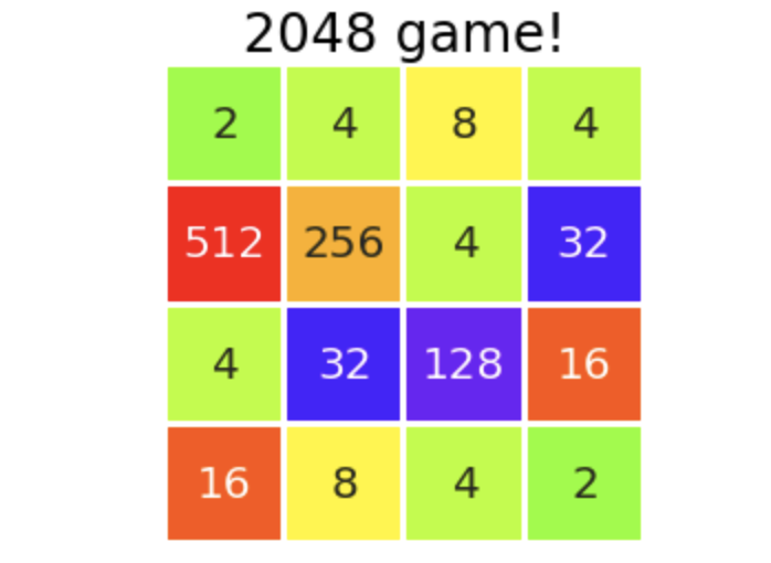
I chose ** 2048 games ** as the learning theme (↓ like this). Do you know
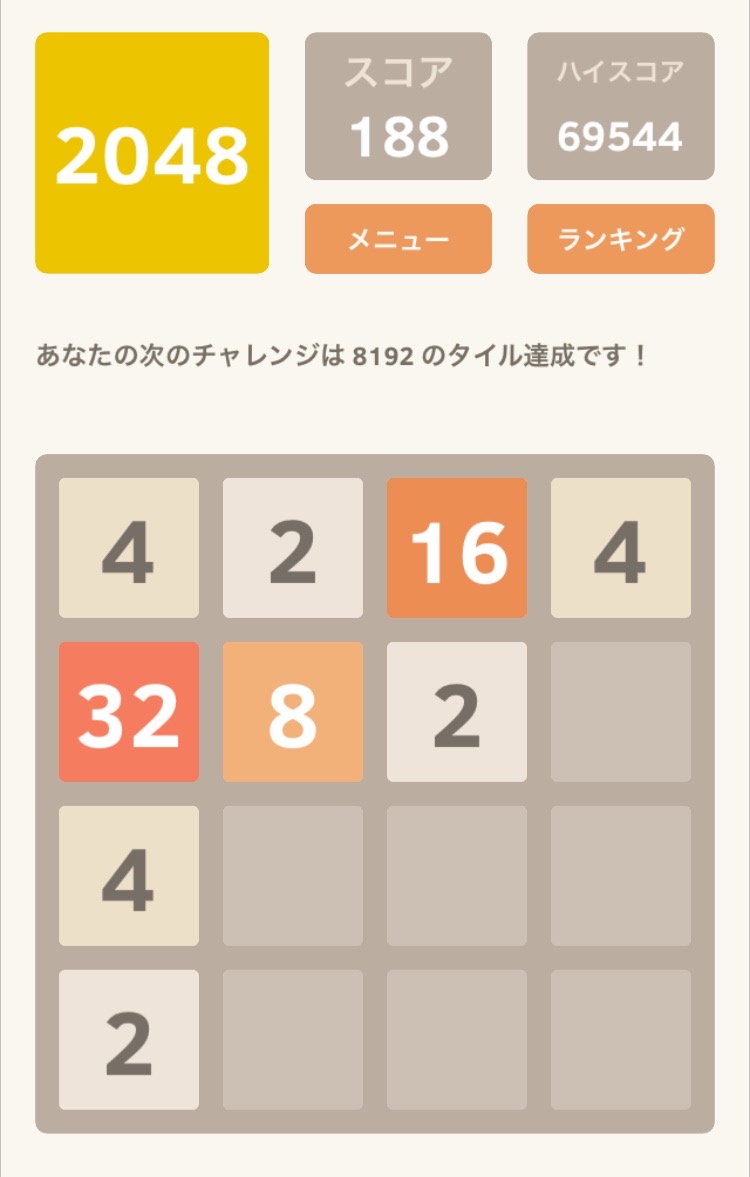
I'll explain the rules later, but it's so easy that you'll understand it. There are many smartphone apps and web versions, so please try it out.
1-1. Rules
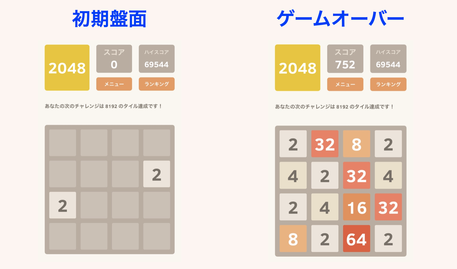
A tile with a power of 2 is placed on the board of 4 $ \ times $ 4 squares. At the beginning of the game, tiles of "2" or "4" are placed in 2 randomly selected squares.
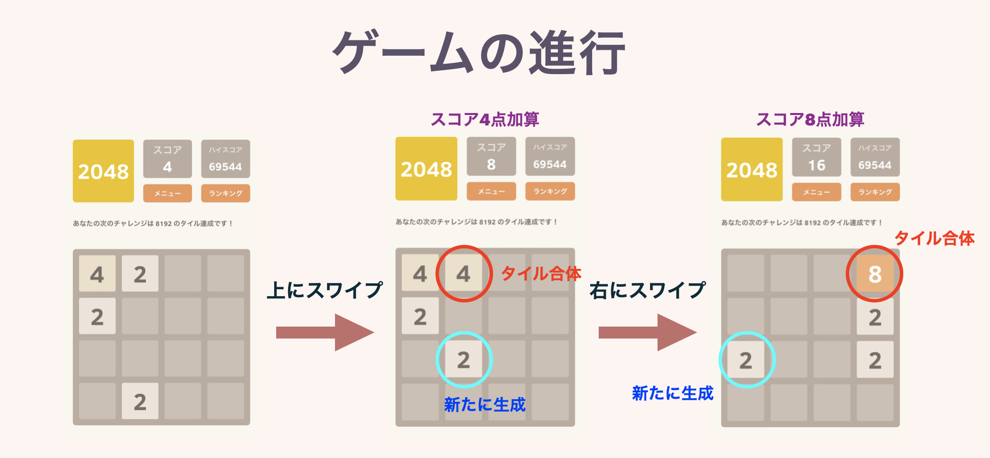
Each turn, the player chooses one of the four directions, up, down, left, and right, and swipes or presses a button. Then, all the tiles on the board slide in that direction. At this time, if tiles with the same number collide, they will merge and the number will increase, forming a single tile. At this time, the numbers written on the tiles created will be added as scores.
At the end of each turn, a new "2" or "4" tile will be created in one of the empty squares. If you can't move in any direction, the game is over. Aim for a high score by then! It is a game called. As the name of this game suggests, the goal is to "make 2048 tiles" at first.
↓ It is an illustration. The rules are really simple.
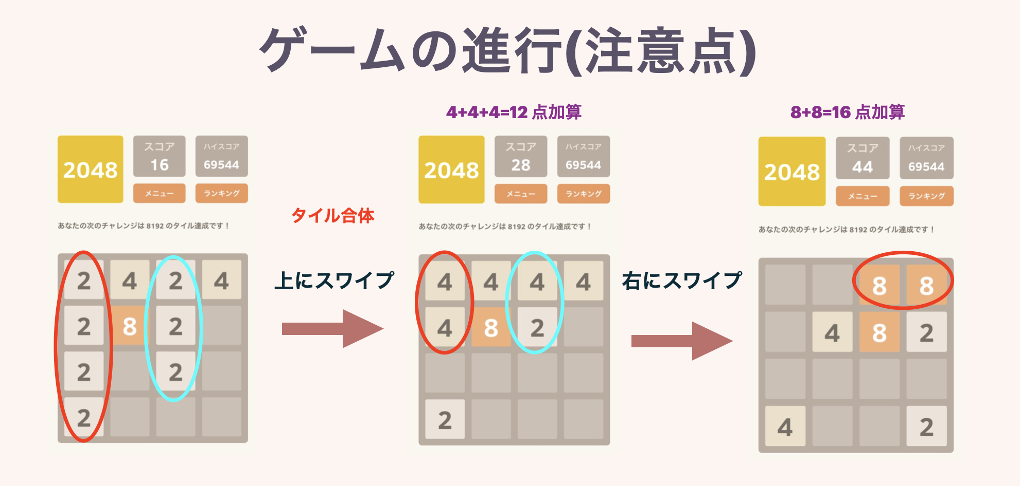
The second figure shows the behavior when three or more tiles with the same number are lined up. If multiple tiles are completed at the same time, the score will be added properly.
1-2. Tips for this game
There is some luck in this game, but the score probably reflects the player's skill. In other words, it is a "game that you can improve by studying and practicing." Later, I will ask AI to practice the game, but I will briefly write down the tips of this game that I got at this timing. It would be great if AI could learn this trick for himself.
However, if you want to experience how much level of AI you can make, ** I recommend you to play it several times without seeing this tip. ** If you know what your initial ability score is, it will be a little easier to understand what level you are at in the future AI learning process. (If you don't mind, you can open it normally.)
Please read this content after understanding the above (click the triangle mark on the left). In this game, at the beginning, it's okay because the tiles merge somewhere no matter how you move it, but eventually the large numbers get in the way and the board becomes narrower and narrower. Therefore, it is very effective to take the policy of ** collecting large numbers in some corners **. (There are various tips on how to collect them in the corner.) In the figure on the left, large numbers are collected in the upper left direction. If you swipe down on this board, "256" and "128" will become obstructive tiles in the middle, and it will become unstable at once (it really goes to the game over at once). ). If you play carefully so as not to lose this shape, you can bring it to the board as shown in the figure on the right. From here you can see that you can go straight to "2048". The moment of collecting tiles at once is the most pleasant point in this game.
1-3. Goal
For the time being, I will set a goal (dream) for this time. The ideal is "AI that can get a higher score than myself". I think I understand this game to some extent, and the high score of 69544 points in the screenshot I showed earlier is quite high, but if AI exceeds this, I will be impressed.
As a guideline for the score, if a person who does not know this game plays for the first time, the game will be over with about 1000 to 3000 points. If you play a few times and get used to the game, you will be able to get about 5000 to 7000 points. (It's just that people around me had this tendency. There aren't many samples, so please use it as a reference). As I will explain later, if you choose your hand completely randomly, you will get only about 1000 points on average.
Now that we've talked about 2048 games, let's get into reinforcement learning!
2. Theoretical armament
Prior to implementation, we will organize the theory that is the basis of this game AI creation ~~ or something ~~. I would like to follow the flow from the basics of reinforcement learning to the DQN used this time. The author will also write step by step while doing obenkyo, so let's do our best together.
2-1. About reinforcement learning
In the first place, reinforcement learning is a field with machine learning, along with supervised learning and unsupervised learning. Reinforcement learning is to define ** agents ** that move around in some environment, proceed with learning processing while repeatedly collecting data, and learn optimal behavior that maximizes the "reward" that can be obtained. It is the flow of. It seems that reinforcement learning is applied to the AI of shogi and go that we often hear, and automatic driving technology.
In the following, I will set the theme of 2048 games, but I will also incorporate a little more technical terms and organize them.
2-1-1. Action Policy
To start reinforcement learning, first define the "** agent " that actually plays the game (it is subtle if it is said that the agent itself was defined in this implementation, but even if it is virtual, the game is defined. I think it's good to be aware of the existence of playing). Also, set " Reward " in the game to give the agent the purpose of "maximizing the reward at the end of the game". How to set the reward is an important factor. Also, during play, the agent encounters various boards and is forced to select the " action " to be taken there. Each board is called " state **" in reinforcement learning terms.
When the agent learning is completed, it means that "the best action a is known for all states s". It is easy to understand if you consider "○ × game" as an example. That game will always be a draw as long as both parties continue to do their best. This means that if you "memorize" all possible states (board), you will be an undefeated ○ × gamemaster without even knowing the extreme rules.
Here we define the term "** behavior policy **". This is a "rule in which the agent selects an action for each state". An agent with a fixed behavior policy plays the game by selecting the next move according to certain rules (well, it is a machine) like a machine. The purpose of reinforcement learning may be rephrased as optimizing this behavioral policy and seeking the optimal behavioral policy. In the example of the ○ × game, following the best moves that should have been memorized is the optimal action policy.
In addition, it seems that it is customary to express the behavior policy with the symbol $ \ pi $.
2-1-2. State value function
I've been learning from a while ago, but I'll start talking about how to learn concretely.
First, define the ** state value function ** $ v_ \ pi (s) $. This is a function that assumes a specific action policy π and takes a state s as an argument. The return value is "the expected value of the total rewards obtained after the present when starting from the state s and continuing to select actions according to the action policy π until the end of the game".
?? It may be, but if you think about it, it's not a big deal. When the action policy is fixed, the value of the state value function represents "how good each board is".
I will show it because it feels better (personally) to use mathematical formulas. All the symbols that appear suddenly give meaning.
Yes, this is the equation that the state value function generally satisfies. This is called the ** Bellman equation **.
-$ p (r, s'\ | \ s, a) $ represents "conditional probability that r is obtained as a reward and transitions to state s'when action a is selected from state s". I will. (Even if you select the same action on the same board, you will not always get the same reward / transition destination, so this measure is taken. For example, in 2048 games, the position of newly generated tiles is random. .) -$ r + v_ \ pi (s') $ is "when a is selected in the first action, the reward r is acquired and the state transitions to the state s', and then the action policy π is followed until the end of the game. , Expected value of the sum of rewards obtained from now ”. -$ \ pi (a \ | \ s) $ represents "conditional probability that action a is selected in state s in action policy π". (If π does not include stochastic action selection, this can be removed.)
To summarize the above, the inner sigma expresses "the expected value of the sum of the rewards that can be obtained from now on when action a is selected from the current state s and then acts according to π". Furthermore, by summing the actions with the outside sigma, it becomes "the expected value of the total reward obtained by the end of the game if the action is continuously selected according to the action policy π from the current state s".
Supplementary information about "discount rate" In the Bellman equation of (1), a parameter called ** discount rate ** is generally introduced (the symbol is γ). However, this time, I decided not to deal with it because the formula is equivalent to (1) because $ \ gamma = 1 $ was set in the implementation part, and the author's understanding is low. sorry.
Equation (1) above shows the calculation method rather than the definition of the state value function. Only one point, if the value of the state value function for the end state (game over board) is defined in advance as 0, the state value function for all states can be traced back to the previous state and the previous state. You can calculate the value of. It is an image that the value of the correct state value function gradually propagates from the end state. In high school mathematics, it is a recurrence formula, and in algorithm, it is ** dynamic programming **.
I will not go deeper into dynamic programming. However, it may be worth keeping in mind that in order to do this calculation, we need to at least run a loop for all states.
Well, we have defined the state value function itself, but in the end, what "learning" does is not yet shown. I will answer that question next.
2-1-3. Behavior-State Value Function
The state value function described above determines whether each state is good or bad on the premise that the behavior policy π is fixed. In other words, it cannot improve the behavior policy π by itself. Here's how to get a better behavioral policy. However, here, the behavior policy is "better". "For any state s, $ v_ {\ pi1} (s) \ leq v_ {\ pi2} (s) $ holds." It is determined that. (Π2 is a "better" behavior policy than π1.)
Very similar in name, but defines a ** behavior-state value function ** $ q_ \ pi (s, a) $. This represents "the expected value of the total reward that can be obtained from now on when action a is selected from the current state s and then the action is continuously selected according to the action policy π". that? As some of you may have thought, this appears entirely in part of equation (1). That is,
is. Using this, Eq. (1) becomes
Can be expressed as.
Now I will make a conclusion at once. How to improve your behavioral policy ** "For all actions a that can be selected in the current state s, refer to the value of the action-state value function $ q_ {\ pi} (s, a) $ and select the action a that maximizes this. "Correct" **.
The bottom line is, "Ignore the current behavioral policy for just one move, look at a different world, and modify the policy to choose the move that looks best." I think you can intuitively understand that if you continue to make this improvement, you will get more and more "better" policies. It is possible to show this mathematically, but it is rather troublesome, so I will omit it here.
2-1-4. Summary so far
I've said a lot, but for the time being, I've settled down, so I'll summarize it briefly. The flow until the agent learns the optimal behavior policy is
--For the time being, set the action policy $ \ pi $ appropriately. --Calculate the state value function $ v_ {\ pi} (s) $ by dynamic programming. --Behavior-The state value function $ q_ {\ pi} (s, a) $ is calculated by Eq. (2). --Create a new action policy $ \ pi'$ by the method described above. --Replace this $ \ pi'$ with the first action policy π and repeat the same operation.
is. By repeating this all the time, the agent can get a better behavior policy. This is the mechanism of "learning" in reinforcement learning.
Supplement: About a little cheated point I talked about the theory that you can learn by repeating the above loop, but when you actually try to calculate, $ p (r, s'\ | \ s, a that appears in (1) and (2) ) You face the question of knowing the value of $. That's fine if you have a complete understanding of the game's specifications (as we programmers) and are theoretically required, but you may not know this when playing an unknown game. I will collect this later by the `2-2-3. TD method`.
2-2. Q-Learning
The algorithm summarized above is undoubtedly the correct learning algorithm, but it has the disadvantage that the policy is not improved until the end of one game, and that "the current behavior policy does not always lead to the end of the game". There is. That's not the case with 2048 games, but this is a big problem when applying it to general games (for example, a maze). The solution to this point is the ** Q-Learning ** algorithm, which was implemented this time and will be explained below.
2-2-1. Off-policy
Only the definition of terms is given here. We aim to improve our behavioral policy, but if you think about it, when an agent plays and collects data, you don't have to collect data according to the current optimal behavioral policy. Therefore, let us consider a method of "moving an agent according to a policy different from the policy to be improved and collecting data". This is called ** off-policy ** data collection.
2-2-2. Greedy policy
I'm a little reminded now, but I'm defining the term ** Greedy Policy **. This is an "action policy that has no stochastic elements and keeps selecting actions." The policy is such that the conditional probability $ \ pi (a \ | \ s) $ that appears in equations (1) and (3) is 1 only for a specific a and 0 for other actions. It can also be rephrased as.
In Greedy policy π, if the state s is defined, one action is fixed, so that action is expressed as $ \ pi (s) $.
At this time, in general,
Is obtained. This is called the ** behavior-Bellman equation for the state value function **. By this formula, the value on the left side is calculated using the reward r when action a is selected in the state s and the state s', $ q_ {\ pi} (s', \ pi (s')) $ of the transition destination. You can try again. Also, with this formula, there is no need to go through the state value function.
The following is an overview of Q-Learning that makes use of equation (5).
2-2-3. TD method
In the algorithm explained at the beginning, it was stated that the policy could not be improved without waiting for the end of one game. On the other hand, there is a method to perform update processing at the moment when data for one turn is collected. This is called the "** TD method (Temporal-Difference method) **", and the TD method that collects data off-policy is called Q-Learning. In this case, AI can be smart while collecting data, and can avoid the situation where the goal of the maze cannot be reached forever.
The update is performed using equation (5). The value of $ p (r, s'\ | \ s, a) $ is initially unknown, an approximate value is calculated from the obtained data, and by collecting the data, the value becomes closer to the true value. At the same time, the value of the action-state value function is also modified.
However, in actual Q-Learning, it seems that the value is corrected by the following formula instead of formula (5). (The feeling of bringing the value of the action-state value function closer to $ r + q_ {\ pi} (s', \ pi (s')) $ remains the same.)
α is a parameter that adjusts the weight of correction, and is called ** learning rate **. (This is completely my expectation, but it is memory to keep and update the value of $ p (r, s'\ | \ s, a) $ for every (s, a) pair. I think there are many cases where it is difficult.)
Yes. I explained it a little loosely towards the end, but to be honest, I didn't use this formula in the implementation part, so I was a little less motivated. Anyway, the important idea is that ** the behavior-state value function is updated while collecting data with the off-policy, and a better behavior policy can be obtained by selecting the action that maximizes this value **. The mechanism of the production algorithm based on this is shown below, and the long theory section is closed.
2-3. DQN
In the theory section, we first explained the basic mechanism of reinforcement learning, and then described a method called Q-Learning that makes it more efficient. However, the current algorithm still has a fatal problem. The point is that the learning process does not end when there are too many possible states.
With conventional algorithms, no matter how underestimated, the number of possible states must be calculated, and the value of the action-state value function must be calculated for all states (of course, this is repeated many times. You will get a better policy). The amount of operations that Python can perform per second is at most $ 10 ^ {7} $ times or so, while the number of states in 2048 games is 16 squares on the board, and it seems to be about $ 12 ^ {16} $. That's right. It seems that learning is never over, considering that it goes around a loop of this length many times. If you start to say the number of states of shogi or go, it will not end forever. (I'm not so familiar with Python's computing speed, so I wrote it down, but it doesn't end for the time being.)
In order to solve this problem, ** DQN ** is to bring out a great ** neural network ** and do Q-Learning. DQN is an acronym for Deep Q Network.
2-3-1. Neural network
Again, I will not follow the detailed theory and mechanism of neural networks in this article. Here, I will describe the minimum world view necessary to understand the learning mechanism of 2048 game AI. (In fact, I'm also an inexperienced person, so I'm sorry I don't know the depth.)
Neural networks are used in ** deep learning **, but to put it plainly, they are "functions". (Multivariable input and multivariable output are the default). Prepare a lot of simple linear functions, pass the input through them, and add some processing. After repeating this operation in multiple layers, the output is output in some form. That is a neural network. By tweaking the number of internal functions, the type of processing, and the number of layers, you can really flexibly transform into various functions. (Hereafter, the neural network is sometimes abbreviated as "NN".)
And neural networks have another important function. That is ** parameter tuning **. Earlier, the contents of NN were fixed and worked as a function, but by giving the output of "correct answer" to NN at the same time as input, the value of the parameter included in the internal function is output so that a value close to the correct answer is output. Can be modified. Neural networks can "learn" so that they become functions with the desired properties.
For the implementation, we will use the framework ** TensorFlow ** this time, so I think it's okay to understand the contents for the time being. Obenkyo will take another opportunity.
2-3-2. Convolutional Neural Network (CNN)
There is a kind of NN called ** convolutional neural network **. This is the kind used for image recognition, etc., and it is better to grasp the characteristics of the two-dimensional spread of the input (just like the board surface) rather than simply giving the input value. So I will use it this time. That's it for the time being.
2-3-3. Incorporate into Q-Learning
The way to use NN is to "create a neural network that calculates the value of the action-state value function from the state and action of the board". It was said that the conventional method of finding $ q_ {\ pi} (s, a) $ for all states / actions was impossible, but if such an NN could be created, it would be "somehow similar". You can expect to be able to choose the best move by looking at the board that says "there is a part that communicates".
I understand it with an expression. As with equations (5) and (6), the purpose of Q-Learning is to update the value of $ q_ {\ pi} (s, a) $. Therefore, the input of NN is also the state of the board itself + the selected action.
Since we want to bring the calculation result closer to $ r + q_ {\ pi} (s', \ pi (s')) $, we use this as the "correct answer value" and perform NN learning processing. Although it is only in the area of "function approximation", it can be expected that the performance (approximation accuracy) will improve steadily by repeating the data collection and learning process.
The above is the whole picture of DQN used this time. I think it's faster to look at the code for the specific story, so I'll post it later.
2-4. Summary of world view
The theory section has become longer than expected (Gachi). Let's reorganize the whole picture here and move on to the implementation part.
--In reinforcement learning, the behavior policy is improved so that the agent plays the game and the reward obtained is maximized. --Behavior-If the value of the state value function can be calculated accurately for every state / action, the best move on all boards is known. ――Q-Learning is to collect data with off-policy and update the value of action-state value function at any time. --If there are too many states, it is uncontrollable as it is, so the behavior-state value function is approximated and calculated using a neural network, and data is collected to perform this NN learning process. (DQN)
Thank you for your hard work! Even if you don't understand well, you may understand it by reading the code, so please go back and forth. I'm sorry if my theory summary is simply not good. At least there should be some missing parts, so if you want to study more properly, I think you should try some other books.
This time the theory is really over. Let's move on to the code ↓ ↓
3. Implementation
Then, I will put more and more code. Perhaps if you stick it from the top, it will be possible to reproduce it (although it is not possible to get the exact same result because it is full of codes involving random numbers). Also, please forgive me if you can see unsightly code in various places.
For the time being, only the items that should be imported are pasted here. Please make all the following codes on this assumption. (Please note that it may actually contain unnecessary modules)
2048.py
import numpy as np
import copy, random, time
from tensorflow.keras import layers, models
from IPython.display import clear_output
import matplotlib.pyplot as plt
import seaborn as sns
import matplotlib
matplotlib.rcParams['font.size'] = 20
import pickle
from tensorflow.keras.models import load_model
3-1. Game class definition
First, implement 2048 games on the code. It's long, but the contents are thin, so please look at it with that intention. It is not limited to this code, but it may be better to look at it because it has a Japanese commentary at the end. Then.
2048.py
class Game:
    def __init__(self):
        self.restart()


    def restart(self):
        self.board = np.zeros([4,4])
        self.score = 0
        y = np.random.randint(0,4)
        x = np.random.randint(0,4)
        self.board[y][x] = 2
        while(True):
            y = np.random.randint(0,4)
            x = np.random.randint(0,4)
            if self.board[y][x]==0:
                self.board[y][x] = 2
                break


    def move(self, a):
        reward = 0
        if a==0:
            for y in range(4):
                z_cnt = 0
                prev = -1
                for x in range(4):
                    if self.board[y][x]==0: z_cnt += 1
                    elif self.board[y][x]!=prev:
                        tmp = self.board[y][x]
                        self.board[y][x] = 0
                        self.board[y][x-z_cnt] = tmp
                        prev = tmp
                    else:
                        z_cnt += 1
                        self.board[y][x-z_cnt] *=2
                        reward += self.board[y][x-z_cnt]
                        self.score += self.board[y][x-z_cnt]
                        self.board[y][x] = 0
                        prev = -1
        elif a==1:
            for x in range(4):
                z_cnt = 0
                prev = -1
                for y in range(4):
                    if self.board[y][x]==0: z_cnt += 1
                    elif self.board[y][x]!=prev:
                        tmp = self.board[y][x]
                        self.board[y][x] = 0
                        self.board[y-z_cnt][x] = tmp
                        prev = tmp
                    else:
                        z_cnt += 1
                        self.board[y-z_cnt][x] *= 2
                        reward += self.board[y-z_cnt][x]
                        self.score += self.board[y-z_cnt][x]
                        self.board[y][x] = 0
                        prev = -1
        elif a==2:
            for y in range(4):
                z_cnt = 0
                prev = -1
                for x in range(4):
                    if self.board[y][3-x]==0: z_cnt += 1
                    elif self.board[y][3-x]!=prev:
                        tmp = self.board[y][3-x]
                        self.board[y][3-x] = 0
                        self.board[y][3-x+z_cnt] = tmp
                        prev = tmp
                    else:
                        z_cnt += 1
                        self.board[y][3-x+z_cnt] *= 2
                        reward += self.board[y][3-x+z_cnt]
                        self.score += self.board[y][3-x+z_cnt]
                        self.board[y][3-x] = 0
                        prev = -1
        elif a==3:
            for x in range(4):
                z_cnt = 0
                prev = -1
                for y in range(4):
                    if self.board[3-y][x]==0: z_cnt += 1
                    elif self.board[3-y][x]!=prev:
                        tmp = self.board[3-y][x]
                        self.board[3-y][x] = 0
                        self.board[3-y+z_cnt][x] = tmp
                        prev = tmp
                    else:
                        z_cnt += 1
                        self.board[3-y+z_cnt][x] *= 2
                        reward += self.board[3-y+z_cnt][x]
                        self.score += self.board[3-y+z_cnt][x]
                        self.board[3-y][x] = 0
                        prev = -1


        while(True):
            y = np.random.randint(0,4)
            x = np.random.randint(0,4)
            if self.board[y][x]==0:
                if np.random.random() < 0.2: self.board[y][x] = 4
                else: self.board[y][x] = 2
                break

        return reward
I decided to let the Game class manage board and score. As the name suggests, it is the board and the current score. board is represented by a two-dimensional numpy array.
By the restart method, tiles of" 2 "are placed at two random places on the board, the score is set to 0, and the game is started. (In the explanation of the rules in Chapter 1, I said that "2" or "4" is placed on the initial board, but only "2" appears in the code. This is when I implemented the Game class. At first, I misunderstood that it was only "2". Please forgive it because it has almost no effect on the game.)
The move method takes the type of action as an argument, changes the board accordingly, and adds the score. As a return value, the score added in this one turn is returned, which will be used later. (In this study, the in-game score was used as it is as the "reward" that the agent gets). Actions are represented by integers from 0 to 3, and are associated with left, top, right, and bottom, respectively. The implementation of board changes is a uselessly long index kneading, probably less readable. You don't have to read it seriously. It may be possible to write more beautifully, but please forgive me here (´ × ω × `)
Also, in the last while loop, one new tile is generated. This may also be an inefficient implementation in terms of algorithm, but I forcibly hit it. I regret it. A tile of "2" or "4" is generated, but as a result of a light statistic by the author, it was about "2 will spring up with an 80% probability", so I implemented it that way. Actually, it may be a little off, but this time we will do it.
Note that the move method assumes that a" selectable "action is input. (Because the direction in which the board does not move cannot be selected during play.) For this, use the following function.
3-2. Judgment of selectable actions
In the future, there will be many situations where you want to know whether each action is "selectable" on each board, such as when inputting to the move method above. Therefore, we prepared ʻis_invalid_action` as a judgment function. Please note that it gives the board and action, and returns True if it is an action that cannot be selected.
Also, this code is very similar to the move method and is just uselessly long, so it is collapsed into the triangle mark below. Please close it as soon as you copy the contents. Because it's not good.
`is_invalid_action`
2048.py
def is_invalid_action(state, a):
    spare = copy.deepcopy(state)
    if a==0:
        for y in range(4):
            z_cnt = 0
            prev = -1
            for x in range(4):
                if spare[y][x]==0: z_cnt += 1
                elif spare[y][x]!=prev:
                    tmp = spare[y][x]
                    spare[y][x] = 0
                    spare[y][x-z_cnt] = tmp
                    prev = tmp
                else:
                    z_cnt += 1
                    spare[y][x-z_cnt] *= 2
                    spare[y][x] = 0
                    prev = -1
    elif a==1:
        for x in range(4):
            z_cnt = 0
            prev = -1
            for y in range(4):
                if spare[y][x]==0: z_cnt += 1
                elif spare[y][x]!=prev:
                    tmp = spare[y][x]
                    spare[y][x] = 0
                    spare[y-z_cnt][x] = tmp
                    prev = tmp
                else:
                    z_cnt += 1
                    spare[y-z_cnt][x] *= 2
                    spare[y][x] = 0
                    prev = -1
    elif a==2:
        for y in range(4):
            z_cnt = 0
            prev = -1
            for x in range(4):
                if spare[y][3-x]==0: z_cnt += 1
                elif spare[y][3-x]!=prev:
                    tmp = spare[y][3-x]
                    spare[y][3-x] = 0
                    spare[y][3-x+z_cnt] = tmp
                    prev = tmp
                else:
                    z_cnt += 1
                    spare[y][3-x+z_cnt] *= 2
                    spare[y][3-x] = 0
                    prev = -1
    elif a==3:
        for x in range(4):
            z_cnt = 0
            prev = -1
            for y in range(4):
                if spare[3-y][x]==0: z_cnt += 1
                elif spare[3-y][x]!=prev:
                    tmp = state[3-y][x]
                    spare[3-y][x] = 0
                    spare[3-y+z_cnt][x] = tmp
                    prev = tmp
                else:
                    z_cnt += 1
                    spare[3-y+z_cnt][x] *= 2
                    spare[3-y][x] = 0
                    prev = -1


    if state==spare: return True
    else: return False
3-3. Visualization of board surface
AI can learn without problems even if there is no function to show the board, but we made it because we humans are lonely. However, the main subject is not here, so I've cut a lot with the excuse.
2048.py
def show_board(game):
    fig = plt.figure(figsize=(4,4))
    subplot = fig.add_subplot(1,1,1)

    board = game.board
    score = game.score
    result = np.zeros([4,4])
    for x in range(4):
        for y in range(4):
            result[y][x] = board[y][x]

    sns.heatmap(result, square=True, cbar=False, annot=True, linewidth=2, xticklabels=False, yticklabels=False, vmax=512, vmin=0, fmt='.5g', cmap='prism_r', ax=subplot).set_title('2048 game!')
    plt.show()

    print('score: {0:.0f}'.format(score))
I reproduced only the minimum functions using a heat map (really the minimum). You don't need to read the details about this, I think you can copy the brain death. Here's what it actually looks like.
Supplement: Conflicts related to heat maps It's a really ridiculous story, but when implementing the 2048 game, there was an idea to "use numbers simply as 1,2,3 ... instead of powers of 2." There is only one reason, because this visualization function colors the board more beautifully. However, in that case, there was no sense of 2048 as a game, and the intuition that it seemed that learning on the board could not be done well worked, so it ended up like this. As a result, as you can see, the small numbers are very close in color and difficult to see. Isn't there a heat map that changes color on the logarithmic axis?
3-4. Play
If you just want to learn, this process is completely unnecessary, but since it's a big deal, let's play the python version 2048 game, so I wrote such a function. This is also quite omission, and you don't have to read it seriously. If you do your best, you can make the UI as comfortable as you want, but it is not the main subject, so I will leave it.
2048.py
def human_play():
    game = Game()
    show_board(game)
    while True:
        a = int(input())
        if(is_invalid_action(game.board.tolist(),a)):
            print('cannot move!')
            continue
        r = game.move(a)
        clear_output(wait=True)
        show_board(game)
Now, if you execute human_play (), the game will start. Enter a number from 0 to 3 to move the board.
The board appears like this and you can play. After all it is hard to see the board. By the way, with this code, the moment you accidentally enter something other than numbers, the game is over with no questions asked. I don't know the UI. Also, since this does not have a game end judgment, if you can not move it, take the previous specification and make strange input to get out of the game. I don't know the UI.
Let's let the computer play this game at this timing.
2048.py
def random_play(random_scores):
    game = Game()
    show_board(game)
    gameover = False
    while(not gameover):
        a_map = [0,1,2,3]
        is_invalid = True
        while(is_invalid):
            a = np.random.choice(a_map)
            if(is_invalid_action(game.board.tolist(),a)):
                a_map.remove(a)
                if(len(a_map)==0):
                    gameover = True
                    is_invalid = False
            else:
                r = game.move(a)
                is_invalid = False
                time.sleep(1)
                clear_output(wait=True)
                show_board(game)
    random_scores.append(game.score)
I told you to let the computer play, but it is a function that allows you to see what happens when you choose a hand completely randomly. Take an appropriate array as an argument (foreshadowing). This argument doesn't matter for viewing, so let's execute it appropriately like random_play ([]). The game progresses like an animation.
As you can see, at this stage, I don't feel like I'm playing with will (it's random, so of course). Therefore, let's grasp the ability (average score, etc.) at this point. I took an array as an argument to do this. In the random_play function, comment out the code related to board visualization (3rd line from the top and 2nd to 4th lines from the bottom), and then execute the following code.
2048.py
random_scores = []
for i in range(1000):
    random_play(random_scores)

print(np.array(random_scores).mean())
print(np.array(random_scores).max())
print(np.array(random_scores).min())
I did a test play 1000 times and checked the average score, the highest score, and the lowest score. Execution ends unexpectedly soon. The result will change slightly depending on the execution, but in my hands
--Average score: ** 1004.676 points ** --Highest score: ** 2832 points ** --Lowest score: ** 80 points **
I got the result. It can be said that this is the power of AI that has not learned anything. So, if you get well above 1000 points on average, you can say that you have learned a little. Also, since the highest score of 1000 plays is about this level, I think that exceeding 3000 points is an area that is difficult to reach with luck alone. Let's consider the learning results later based on this area.
3-5. Creating a neural network
Here, we implement a neural network, which is the person who calculates the value of the behavior-state value function and also receives the collected data for learning. However, all of this troublesome part takes the form of a round throw in ** TensorFlow **, so you can think of the black box as a black box. For the time being, stick the code.
2048.py
class QValue:
    def __init__(self):
        self.model = self.build_model()

    def build_model(self):
        cnn_input = layers.Input(shape=(4,4,1))
        cnn = layers.Conv2D(8, (3,3), padding='same', use_bias=True, activation='relu')(cnn_input)
        cnn_flatten = layers.Flatten()(cnn)

        action_input = layers.Input(shape=(4,))

        combined = layers.concatenate([cnn_flatten, action_input])
        hidden1 = layers.Dense(2048, activation='relu')(combined)
        hidden2 = layers.Dense(1024, activation='relu')(hidden1)
        q_value = layers.Dense(1)(hidden2)

        model = models.Model(inputs=[cnn_input, action_input], outputs=q_value)
        model.compile(loss='mse')
        return model

    def get_action(self, state):
        states = []
        actions = []
        for a in range(4):
            states.append(np.array(state))
            action_onehot = np.zeros(4)
            action_onehot[a] = 1
            actions.append(action_onehot)

        q_values = self.model.predict([np.array(states), np.array(actions)])
        times = 0
        first_a= np.argmax(q_values)
        while(True):
            optimal_action = np.argmax(q_values)
            if(is_invalid_action(state, optimal_action)):
                q_values[optimal_action][0] = -10**10
                times += 1
            else: break

            if times==4:
                return first_a, 0, True #gameover

        return optimal_action, q_values[optimal_action][0], False #not gameover
It is implemented in the form of QValue class. This instance becomes the learning target itself (to be exact, its member variable model). And the build_model method in the first half is a function that is executed at the time of instantiation and creates a neural network.
I will give an overview of the build_model method, but I will not explain each" NN word "in detail. Hmmm, I think it's okay. I think it is worth reading if you are knowledgeable. (At the same time, there may be room for improvement. Please teach me ...)
We will use the convolutional neural network (CNN) that we talked about in Theory. This is because I expected to capture the two-dimensional expanse of the board. As input, we take a 4x4 array that corresponds to the board surface and an array of length 4 that corresponds to the selection of actions. Action selection is performed by ** One-hot encoding **, in which one of the four locations is represented by an array of 1 and the rest is represented by an array, instead of inputting 0 to 3. Eight types of 3x3 filters are used for convolution. It also specifies the padding, bias, and activation function. As hidden layers, we prepared one layer with 2048 neurons and one layer with 1024 neurons, and finally defined the output layer. ReLU is used as the activation function of the hidden layer. In addition, the least squares error is adopted as the error function used for parameter tuning.
The explanation about NN is rounded up here. Even if you don't understand at all, it's okay if you just think that you have defined NN, although you don't know the contents.
There is another method called get_action. This corresponds to the step of "calculating the value of the behavior-state value function with a neural network". Taking the board state state as an argument, prepare one-hot expressions for four types of actions, and insert four inputs into the NN. You can do this with the predict method that comes with tensorflow. As the output of NN, the value of the action-state value function for the four types of actions in state is returned. The general role of this method is to get the action with the largest value with the np.argmax function.
I'm messing up in the second half, but this is checking whether the action selected from the value of the action-state value function can be selected (movable) on the board. If this is not possible, then reselect the action that increases the value of the action-state value function. By the way, this method also determines that the game is over. There are three return values of the get_action method, but in order," the selected action, the action for that board / action-the value of the state value function, and whether the board is game over or not ".
3-6. Play the game based on learning
I tried to play it completely randomly earlier, but this time I will play it by incorporating the learning results. The following get_episode function will play one game. (In reinforcement learning, one game is often called ** episode **.)
2048.py
def get_episode(game, q_value, epsilon):
    episode = []
    game.restart()

    while(True):
        state = game.board.tolist()
        if np.random.random() < epsilon:
            a = np.random.randint(4)
            gameover = False
            if(is_invalid_action(state, a)):
                continue
        else:
            a, _, gameover = q_value.get_action(state)

        if gameover:
            state_new = None
            r = 0
        else:
            r = game.move(a)
            state_new = game.board.tolist()
        episode.append((state, a, r, state_new))

        if gameover: break

    return episode
Prepare an array called ʻepisode, play one game, make one set of "current state, selected action, reward obtained at that time, state of transition destination", and store it in the array more and more. That is the basic operation. The data collected here will be used for later learning processing. To select an action, use the q_value.get_action` method defined earlier. This will select the best move on the spot (and with your current abilities). In addition, the end of the episode is detected by making use of the game over judgment performed by this method.
One thing to note is that "it does not always follow the learning results every turn." The get_episode function takes an argument of ʻepsilon`, which is the" probability of randomly selecting an action during play without following the learning result ". By mixing random action selections, you can learn more diverse boards and expect to become a smarter AI.
In this way, the action policy that "basically selects an action with the Greedy policy, but mixes random actions with a probability of $ \ epsilon $" is called the ** ε-Greedy policy **. How much to set the value of ε is an important and difficult issue. (Usually it is about 0.1 to 0.2.)
This function can also be played with the Greedy policy by setting ʻepsilon = 0. In other words, it is a play of "AI's full power" at that time, not including random actions. The function show_sample` for measuring the ability of AI is shown below.
2048.py
def show_sample(game, q_value):
    epi = get_episode(game, q_value, epsilon=0)
    n = len(epi)
    game = Game()
    game.board = epi[0][0]
#     show_board(game)
    for i in range(1,n):
        game.board = epi[i][0]
        game.score += epi[i-1][2]
#         time.sleep(0.2)
#         clear_output(wait=True)
#         show_board(game)
    return game.score
However, the basic is to execute the get_episode function under ʻepsilon = 0, and after that, the board is reproduced using the episode recording. It's like following a game record in shogi. There is a commented out part in the function, but if you cancel this, you can see it with animation. (As with the random_play function, you can control the speed of the animation by adjusting the value given to time.sleep.) The final score is output as the return value. By using this, you can roughly grasp the learning result by inserting show_sample` between the learning processes.
Now let's implement the learning algorithm!
3-7. Learning process
Define a function train that trains NN. It's a little long, but it's not that difficult, so please read it calmly. I will explain it a little carefully.
2048.py
def train(game, q_value, num, experience, scores):
    for c in range(num):
        print()
        print('Iteration {}'.format(c+1))
        print('Collecting data', end='')
        for n in range(20):
            print('.', end='')
            if n%10==0: epsilon = 0
            else: epsilon = 0.1

            episode = get_episode(game, q_value, epsilon)
            experience += episode

        if len(experience) > 50000:
            experience = experience[-50000:]

        if len(experience) < 5000:
            continue

        print()
        print('Training the model...')
        examples = experience[-1000:] + random.sample(experience[:-1000], 2000)
        np.random.shuffle(examples)
        states, actions, labels = [], [], []
        for state, a, r, state_new in examples:
            states.append(np.array(state))
            action_onehot = np.zeros(4)
            action_onehot[a] = 1
            actions.append(action_onehot)

            if not state_new:
                q_new = 0
            else:
                _1, q_new, _2 = q_value.get_action(state_new)

            labels.append(np.array(r+q_new))

        q_value.model.fit([np.array(states), np.array(actions)], np.array(labels), batch_size=250, epochs=100, verbose=0)

        score = show_sample(game, q_value)
        scores.append(score)
        print('score: {:.0f}'.format(score))
There are five arguments, in order: "Game class instance game, model to be trained (QValue instance) q_value, number of times to learn num, array to store the collected data ʻexperience, learning result It is an array scores`" to put (scores). Follow up for details.
The loop is rotated by the amount of num. Here, "one-time learning" is completely different from one-game play. I will explain the flow of one learning.
Learning is divided into two steps: data collection and NN update. In the data collection part, the get_episode function is activated 20 times (in short, the game is played 20 times). Basically, data is collected by the ε-Greedy policy of ε = 0.1, but only twice out of 20 times, play with the Greedy policy (ε = 0) that does not mix random actions and collect the data. By mixing the two types of play in this way, it seems that it will be easier to learn a wide range of boards and incorporate the board when the game progresses for a long time into the learning.
All collected data will be placed in ʻexperience`. If the length of this array exceeds 50000, the oldest data will be deleted. Also, the next model update step is skipped until 5000 data are collected.
To update the model, extract the data from ʻexperience and create a new ʻexample array. At that time, 1000 pieces are randomly selected from the latest data and 2000 pieces are randomly selected from the remaining part and shuffled. By doing this, it seems that the learning results are less likely to be biased while incorporating new data into the learning.
In the next for statement, we will look at the contents of ʻexampleone by one. For NN learning, it is more efficient in terms of calculation speed to input all at once than to receive each data individually, so we will prepare for it. Instates, ʻactions, and labels, enter the current board, the one-hot expression of the action to be selected, and the "correct" value of the action-state value function at that time.
Regarding the value of the correct answer, this is set as $ r + q_ {\ pi} (s', \ pi (s')) $ as explained in the theory edition 2-2-3. TD method. By doing so, the output of NN will be modified to approach here. This is equivalent to r + q_new in the code. q_new is the" expected value of the reward that will be obtained if you act according to the current policy from the transition destination state, "this is the second state when the next state is given to the q_value.get_action method. Since it corresponds to the output (the next state and the action for the best move there-the value of the state value function), it is acquired as such. In addition, q_new is set to 0 for the game over state.
The NN trains with the following q_value.model.fit method. Please leave this content separately. The NN inputs states and ʻactions are given as arguments, and labelsare given as correct values. You don't have to worry aboutbatch_size and ʻepochs, but setting these values will affect the accuracy of your learning (I'm not entirely sure this is the right setting). verbose = 0 only suppresses unnecessary log output.
After the learning process by the fit method is completed, start the show_sample function and have AI play with full power. While outputting the final score as a log, it is stored in the scores array and used later to calculate the average score etc. The above is the whole picture of "one learning". The train function repeats this.
Supplement: About `batch_size` and ʻepochs` I said that you don't have to worry about these, but I think it's worth knowing just the outline, so I'll organize them lightly. In NN learning, input data is not learned all at once, but is divided into small batches called ** mini-batch **, and then each batch is learned. The size of this batch is `batch_size`. In the above code, the input size is 3000 and batch_size is 250, so it is divided into 12 mini-batch. Then, the learning process is performed once for all the input data, which is counted in the unit of ** epoch **. In the above code, 3000 inputs and 12 batches will make 1 epoch. The parameter ʻepochs` indicates how many epochs the learning process should be repeated. Since epochs = 100 is set here, the flow of batch division → learning for all is repeated 100 times. It's a rough summary, but neural networks are difficult \ (^^) /
4. Learning execution & observation
This is the end of the implementation of the model / function. After that, let's actually learn and see how it grows! I also write articles easily ...
Caution: About the learning results shown here It's as if the code you executed and the result are posted in the article as it is, but in reality, the learning process is partially different because you proceeded with the learning while tinkering and modifying it. (Specifically, the data was collected with ε = 0.2 for the first 30 times, and in the old days, the specifications of the `get_action` method were slightly different. The data may be blown off in the middle). Please note that only. In addition, the output of 10 learnings shown immediately after this is supplemented by re-executing the code later (the output at that time was blown away), and it is different from the learning record of the model to be considered in the future. .. Don't take a closer look> <
4-1. Try to train
First, create an instance of the Game class and the QValue class, and others.
2048.py
game1 = Game()
q_value1 = QValue()
exp1 = []
scores1 = []
The numbering of 1 has no particular meaning. Somehow. With this, the preparation for learning is complete. Let's start the train function.
2048.py
%%time
train(game1, q_value1, 10, exp1, scores1)
Only this. This will do 10 learning sessions. The %% time on the first line is like a magic command and measures the time taken to execute. The reason for doing that is that learning takes a lot of time. It takes about 30 minutes just for these 10 times. However, since the train function is implemented so that the progress status is output at any time, it is easier than going through the unseen darkness. Let's take a leisurely look at the output.
Iteration 1
Collecting data....................
Iteration 2
Collecting data....................
Iteration 3
Collecting data....................
Training the model...
score: 716

Iteration 4
Collecting data....................
Training the model...
score: 908

Iteration 5
Collecting data....................
Training the model...
score: 596
...
Like ʻIteration 3, you can immediately see how many loops you are currently looping. The data collection part is displayed while Collecting data ...is displayed, and the model update part is displayed whileTraining the model ... is displayed. In the first two times, the length of ʻexp1 has not reached 5000 and the model update is skipped.
At the end of each learning, one game is played without random actions and the score is displayed. This result is stored in scores1, so you can collect statistics later.
All you have to do is repeat this. Execute the following code to perform an additional 90 learnings.
2048.py
%%time
train(game1, q_value1, 90, exp1, scores1)
ʻExp1andscores1` are reused, and learning proceeds completely from the previous continuation.
As you can see, this learning really takes time. In my environment, it seems like 5 to 6 hours per 100 times. Recently, Mac-kun was groaning all night while I was sleeping. If you are interested, you can have the same experience by finding time and proceeding with the calculation.
Assuming that 100 learnings have been completed, let's plot the changes in the "full power score" during that period. Use scores1.
2048.py
x = np.arange(len(scores1))
plt.plot(x, scores1)
plt.show()
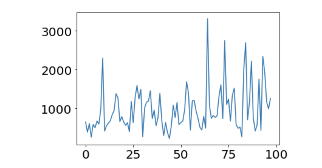
Hmm. It's hard to say that this is a little learned. The average score was 974.45. It's not growing at all. It seems that a little more learning is needed.
4-2. Temporarily save the learning results
This learning is likely to be a long journey, so let's establish only the preservation method. You can save ʻexp1 and scores1` with a function called ** pickle ** in python. Pickle cannot be used for the tensorflow model, but the save function is originally provided. The code is shown below, so save it with a descriptive name.
2048.py
wfile = open('filename1.pickle', 'wb')
pickle.dump(exp1, wfile)
pickle.dump(scores1, wfile)
wfile.close()
q_value1.model.save('q_backup.h5')
To retrieve the saved object, do the following.
2048.py
myfile = open('filename1.pickle', 'rb')
exp1_r = pickle.load(myfile)
scores1_r = pickle.load(myfile)

q_value1_r = QValue()
q_value1_r.model = load_model('q_backup.h5')
The r after the name is meant to be an acronym for restore. q_value1 saves the model in it, not the QValue instance, so after creating only the instance, load the model and replace it. The Game class instance is not specially learned, so you can create a new one when you need it.
It is recommended to keep a record of learning diligently like this. Not only can it be a countermeasure when data flies in the middle, but it is also possible to pull the model in the middle of learning later and compare the performance. (I regret not doing this.)
4-3. Repeat train
I felt that the model trained 100 times was still inexperienced, so I just turned the train function. From the conclusion, I had them learn 1500 times. It takes about 4 days even non-stop, so be prepared if you want to imitate ...
For the time being, I briefly analyzed the scores for 1500 times. The scores were learned 100 times each, and the score band was divided by 1000 points, and the table shows whether the scores for each score band were obtained. I also calculated the average score, so I will arrange them. It's not easy to explain in words, so I'll stick the table. (For reference, I will also post the score distribution of Tokizoya's completely random 1000 times play.)
| Number of learning | 0000~ | 1000~ | 2000~ | 3000~ | 4000~ | 5000~ | average |
|---|---|---|---|---|---|---|---|
| random | 529 | 415 | 56 | 0 | 0 | 0 | 1004.68 |
| 1~100 | 61 | 30 | 6 | 1 | 0 | 0 | 974.45 |
| 101~200 | 44 | 40 | 9 | 6 | 1 | 0 | 1330.84 |
| 201~300 | 33 | 52 | 12 | 1 | 0 | 0 | 1234.00 |
| 301~400 | 35 | 38 | 18 | 7 | 2 | 0 | 1538.40 |
| 401~500 | 27 | 52 | 18 | 3 | 0 | 0 | 1467.12 |
| 501~600 | 49 | 35 | 11 | 4 | 1 | 0 | 1247.36 |
| 601~700 | 23 | 50 | 20 | 5 | 2 | 0 | 1583.36 |
| 701~800 | 45 | 42 | 11 | 2 | 0 | 0 | 1200.36 |
| 801~900 | 38 | 42 | 16 | 4 | 0 | 0 | 1396.08 |
| 901~1000 | 19 | 35 | 40 | 4 | 0 | 2 | 1876.84 |
| 1001~1100 | 21 | 49 | 26 | 3 | 1 | 0 | 1626.48 |
| 1101~1200 | 22 | 47 | 18 | 13 | 0 | 0 | 1726.12 |
| 1201~1300 | 18 | 55 | 23 | 4 | 0 | 0 | 1548.48 |
| 1301~1400 | 25 | 51 | 21 | 2 | 1 | 0 | 1539.04 |
| 1401~1500 | 33 | 59 | 7 | 1 | 0 | 0 | 1249.40 |
HM. How about that. As the learning progresses, the average score gradually increases. One line of 3000 points, which could not be reached even once in 1000 random plays, has come out so much after a little learning. For the time being, it can be said that "learning scars are left behind."
Also, when I was watching AI-kun's play after learning, I felt some kind of intention unlike before (well, humans just found regularity on their own). It may be difficult to understand if it is only the momentary board surface, but I will introduce it because I have cut out the scene.
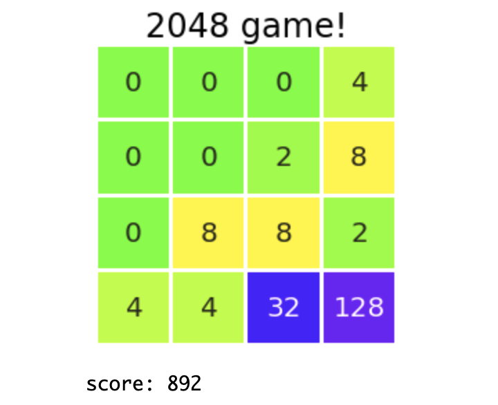
There are many rough edges, but there was a policy of collecting a large number in the lower right corner. This is the same method I introduced in 1-2. Tips for this game. It's interesting that I've been able to learn this trick even though I didn't implement it like "learn to collect big numbers in the corner" from here. Personally, I was quite impressed.
However, the reality is that it is still difficult to get more than 4000 points. I stopped learning at 1500 times simply because it was only a matter of time and, as you can see, the score seemed to stop growing. Actually, I don't know, but I felt that even if I continued to apply the same learning algorithm as it was, I couldn't expect much improvement in performance.
The reason why the score did not increase in the second half, but rather it was depressed, may be due to bad luck, but I felt that the performance had deteriorated normally. To put it a little more properly, I'm guessing that the quality of the contents of the data ʻexperience` used for learning has deteriorated (the advanced board has fallen into a vicious circle where learning is not so much). Anyway, I don't think that the model after 1500 learning is the strongest at present.
Looking closely at the table above, I chose "the model at the end of 1200 learning" as the provisional strongest AI. Well, it's 50 steps and 100 steps. It was good to keep it frozen. The reason why I chose the strongest is because I will implement "an algorithm that seems to choose a better move while keeping the trained model as it is".
That's why I'll load the model at this time. Let's have this child do his best.
2048.py
game1200 = Game()
q_value1200 = QValue()
q_value1200.model = load_model('forth_q_value1_1200.h5')
- Since I just saved the model with this name, it is usually impossible to paste this code in solid. In the future, it is currently impossible to reproduce unless you proceed with learning in your own environment and create a model. sorry. It's a hassle to share the trained model somewhere, but I wonder if there is demand ...
4-4. 1 Read the minions
There is no learning in the future. Keeping the NN model as it is, we will create an action policy that will allow us to play the game better. (I'm sorry to say that the code is over. There are still more.)
Until now, the behavior policy was to "calculate the value of the action-state value function for all actions and select the action that maximizes it" for the given state. This is the process that was done by the get_action method. We will improve this and implement an algorithm that "reads one more move in the next state and selects the best move". First, paste the code.
2048.py
def get_action_with_search(game, q_value):
    update_q_values = []
    for a in range(4):
        board_backup = copy.deepcopy(game.board)
        score_backup = game.score
        state = game.board.tolist()

        if(is_invalid_action(state, a)):
            update_q_values.append(-10**10)
        else:
            r = game.move(a)
            state_new = game.board.tolist()
            _1, q_new, _2 = q_value.get_action(state_new)
            update_q_values.append(r+q_new)
        game.board = board_backup
        game.score = score_backup

    optimal_action = np.argmax(update_q_values)
    if update_q_values[optimal_action]==-10**10: gameover = True
    else: gameover = False

    return optimal_action, gameover
It is a function that replaces the conventional get_action method, get_action_with_search. Turn the for loop for the four actions. From the current state, first select action a once to transition to the next state. Hold the reward r at this time, and consider the next move from the next state. This is q_value.get_action (state_new). This method returns the value of the action-state value function for the best action as the second output, so we receive it as q_new. Here, r + q_new is" the sum of the reward obtained by selecting action a from the current state and the action from the transition destination-the maximum value of the state value function. " The mechanism of this function is to find this value for four types of action a and select the action that maximizes it. (The game over judgment is also performed at the same time.)
Since this policy reads one move rather than a metaphor, it can be expected that the accuracy of selecting the best move will be higher than that of the conventional action selection. Include get_action_with_search in other functions as well.
`get_episode2`
2048.py
def get_episode2(game, q_value, epsilon):
    episode = []
    game.restart()

    while(True):
        state = game.board.tolist()
        if np.random.random() < epsilon:
            a = np.random.randint(4)
            gameover = False
            if(is_invalid_action(state, a)):
                continue
        else:
#             a, _, gameover = q_value.get_action(state)
            a, gameover = get_action_with_search(game, q_value)

        if gameover:
            state_new = None
            r = 0
        else:
            r = game.move(a)
            state_new = game.board.tolist()
        episode.append((state, a, r, state_new))

        if gameover: break

    return episode
`show_sample2`
2048.py
def show_sample2(game, q_value):
    epi = get_episode2(game, q_value, epsilon=0)
    n = len(epi)
    game = Game()
    game.board = epi[0][0]
#     show_board(game)
    for i in range(1,n):
        game.board = epi[i][0]
        game.score += epi[i-1][2]
#         time.sleep(0.2)
#         clear_output(wait=True)
#         show_board(game)
    show_board(game)
    print("score: {}".format(game.score))
    return game.score
That said, it's exactly the same except that the action selection function is really replaced, so I'll fold it. Please close it as soon as you see the contents and understand.
This is really the end of scratching. Finally, check the results and finish!
4-5. Final result
I will bring you q_value1200, who was certified as the provisional strongest a while ago. I asked this child to play 100 times with all his might, and analyzed it as if he had done it in 4-3. Repeat train (I will post it later).
2048.py
scores1200 = []
for i in range(100):
    scores1200.append(show_sample(game1200, q_value1200))
Furthermore, using the same model, we asked them to play 100 times using the one-hand look-ahead algorithm.
2048.py
scores1200_2 = []
for i in range(100):
    scores1200_2.append(show_sample2(game1200, q_value1200))
Organize the results.
| model | 0000~ | 1000~ | 2000~ | 3000~ | 4000~ | 5000~ | 6000~ | average |
|---|---|---|---|---|---|---|---|---|
| Normal | 15 | 63 | 17 | 5 | 0 | 0 | 0 | 1620.24 |
| 1 Look-ahead | 5 | 41 | 32 | 11 | 6 | 2 | 3 | 2388.40 |
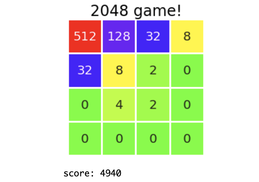
Yes. The conventional algorithm has the same performance as the models we saw before, but the one who introduced the one-hand look-ahead has clearly improved the performance. happy. Especially, it is good that there is a potential to aim for a high score if the flow is good, with 3 times exceeding 6000 points. The highest score out of 100 times was ** 6744 points **. The final board at that time is placed.
It's the last, so it's disturbed, but it seems that we can play at that level, even if we humans do it, we will lose the doggy. I haven't reached the goal of "getting a higher score than myself" that I set a long time ago, but I'm going to stop the improvement around here for the time being. Summer vacation is over. (No, my high score of 69544 isn't too strong ...?)
5. Conclusion
Thank you for your hard work! (If you'd like to read this far, thank you very much. I'm sorry I wrote it for a long time on my side.
Looking back, I really wanted to improve the performance a little more. It's not bad for a high score, but on average, it's only as intelligent as a human first-time play ...
Actually, I was thinking of considering the improvement plan from here a little more, but it seems that it will be too long and the class will start suddenly from tomorrow (currently 3:00 AM), so it is about writing notes. I will pass it to myself in the future.
--Simply repeat the learning a little more. (I think it's a little tough, but ...)
--Try changing the value of ʻepsilon. (I don't know if it will be raised or lowered. However, it may be worth trying to make ε smaller as the learning progresses.) --Increase the length of ʻexperience and ʻexample? I will try. (As learning progresses, one episode becomes longer. The current situation may not be very appropriate.) --Try to divide the board input to CNN into tiles instead of grouping them together. (I think this is quite promising. At present, NN may not be able to distinguish between "2" and "4" tiles. Concerns. Probably the amount of calculation will increase, but the meaning is clear for each tile. Because they are different, I feel that they should be entered separately.) --Tweak batch_size and ʻepochs. (This is a lack of understanding, but it affects the learning accuracy ... I don't feel like I can find an appropriate value.)
――Let's learn how you (the author) are playing. (It seems to be quite annoying in terms of time, but it seems to produce results. I hear that shogi and other professional game records are being learned. Can it be implemented well ...)
――Read and play further. (Well, but I don't know ... the feeling is bad)
Is it roughly like this? At best, it's a plan that I can think of because of lack of self-study and study, so I would be very happy if you could tell me that I should try this more. (On the contrary, please try these improvement plans on my behalf.)
When I put it all together seriously so far, I am very glad that the theory that I intended to understand once came up with hoihoi mistakes and new discoveries. Also, if you do free research with bullets someday, you may write an article like this, so please wait for the new work. We may pursue 2048 game AI a little more.
That's really it. If you find it interesting, please go deeper into the world of reinforcement learning!
The end
I missed the end of summer vacation for only one day. Forgive me.
Recommended Posts