I wrote a summary of Cross Validation, hyperparameter determination, ROC curve, AUC, etc., and an execution demo in Python in relation to the sober but important "model evaluation / index".

This article is the 7th day of Qiita Machine Learning Advent Calendar 2015. When I looked at it, 12/7 was free, so I wrote it in a hurry: grin:

The full code can be found in the GitHub repository here [https://github.com/matsuken92/Qiita_Contents/blob/master/Model_evaluation/Model_evaluation.ipynb).

0. Dataset "Titanic"

Use the familiar Titanic dataset. Data on survivors of the cruise ship Titanic, often used as demonstration data for classification.

First of all, preprocessing and data import

I have a dataset in seaborn, so I'll use that.

%matplotlib inline
import numpy as np
import pandas as pd
from time import time
from operator import itemgetter

import matplotlib as mpl
import matplotlib.pyplot as plt
from tabulate import tabulate
import seaborn as sns
sns.set(style="whitegrid", color_codes=True)

from sklearn import cross_validation
from sklearn import datasets
from sklearn import svm
from sklearn.ensemble import RandomForestClassifier
from sklearn.cross_validation import cross_val_score
from sklearn import grid_search

from sklearn.cross_validation import KFold
from sklearn.cross_validation import StratifiedKFold

from sklearn.metrics import classification_report, roc_auc_score, precision_recall_curve, auc, roc_curve

titanic = sns.load_dataset("titanic")

This is the data. The first 5 lines are displayed.

headers = [c for c in titanic.columns]
headers.insert(0,"ID")
print tabulate(titanic[0:5], headers, tablefmt="pipe")

ID	survived	pclass	sex	age	sibsp	fare	embarked	class	who	adult_male	deck	embark_town	alive	alone
0	0	3	male	22	1	7.25	S	Third	man	1	nan	Southampton	no	0
1	1	1	female	38	1	71.2833	C	First	woman	0	C	Cherbourg	yes	0
2	1	3	female	26	0	7.925	S	Third	woman	0	nan	Southampton	yes	1
3	1	1	female	35	1	53.1	S	First	woman	0	C	Southampton	yes	0
4	0	3	male	35	0	8.05	S	Third	man	1	nan	Southampton	no	1

#Make categorical variables dummy variables
def convert_dummies(df, key):
    dum = pd.get_dummies(df[key])
    ks = dum.keys()
    print "Removing {} from {}...".format(ks[0], key)
    dum.columns = [key + "_" + str(k) for k in ks]  
    df = pd.concat((df, dum.ix[:,1:]), axis=1)
    df = df.drop(key, axis=1)
    return df

titanic = convert_dummies(titanic, "who")
titanic = convert_dummies(titanic, "class")
titanic = convert_dummies(titanic, "sex")
titanic = convert_dummies(titanic, "alone")
titanic = convert_dummies(titanic, "embark_town")
titanic = convert_dummies(titanic, "deck")
titanic = convert_dummies(titanic, "embarked")

titanic['age'] = titanic.age.fillna(titanic.age.median())
titanic['adult_male'] = titanic.adult_male.map( {True: 1, False: 0} ).astype(int)
titanic['alone'] = titanic.adult_male.map( {True: 1, False: 0} ).astype(int)

#Drop unused variables
titanic = titanic.drop("alive", axis=1)
titanic = titanic.drop("pclass", axis=1)

1. Dataset split

1-1. Holdout method

The supervised data that we have at a certain rate is divided into "training data" and "test data" for learning and evaluation. For example, if the ratio of training data to test data is 80:20, it looks like this.

#Training data(80%),test data(20%)Divide into
target = titanic.ix[:, 0]
data = titanic.ix[:, [1,2,3,4,5,6,7,8,9,10,11,12,14]]
X_train, X_test, y_train, y_test = cross_validation.train_test_split(data, target, test_size=0.2, random_state=None)

print [d.shape for d in [X_train, X_test, y_train, y_test]]

`out`


[(712, 23), (179, 23), (712,), (179,)]

The more training data, the higher the learning accuracy, but the lower the model evaluation accuracy.
Increasing the amount of test data increases the accuracy of model evaluation but decreases the accuracy of learning.

Pay attention to the trade-off and decide the ratio.

# SVM(Linear kernel)Classify by and calculate the error rate
clf = svm.SVC(kernel='linear', C=1).fit(X_train, y_train)
print u"Reassignment error rate:", 1 - clf.score(X_train, y_train)   
print u"Holdout error rate:", 1 - clf.score(X_test, y_test)

`out`


Reassignment error rate: 0.162921348315
Holdout error rate: 0.212290502793

# SVM(rbf kernel)Classify by and calculate the error rate
clf = svm.SVC(kernel='rbf', C=1).fit(X_train, y_train)
print u"Reassignment error rate:", 1 - clf.score(X_train, y_train)   
print u"Holdout error rate:", 1 - clf.score(X_test, y_test)

`out`


Reassignment error rate: 0.101123595506
Holdout error rate: 0.268156424581

1-2. Cross Validation (CV): Stratified k-fold

K-fold First, about the simple K-fold. Consider the case where there are 30 pieces of data. n_folds is the number of divisions, divides the data set you have now by the number of divisions, and outputs all combinations in the form of a subscript list as shown below, which is the test data.

 # KFold
# n_Divide the data by the numerical value specified by folds. n_folds=If it is 5, it is divided into 5
#Then, one of them is used as test data, and five patterns are generated.
kf = KFold(30, n_folds=5,shuffle=False)
for tr, ts in kf:
    print("%s %s" % (tr, ts))

`out`


[ 6  7  8  9 10 11 12 13 14 15 16 17 18 19 20 21 22 23 24 25 26 27 28 29] [0 1 2 3 4 5]
[ 0  1  2  3  4  5 12 13 14 15 16 17 18 19 20 21 22 23 24 25 26 27 28 29] [ 6  7  8  9 10 11]
[ 0  1  2  3  4  5  6  7  8  9 10 11 18 19 20 21 22 23 24 25 26 27 28 29] [12 13 14 15 16 17]
[ 0  1  2  3  4  5  6  7  8  9 10 11 12 13 14 15 16 17 24 25 26 27 28 29] [18 19 20 21 22 23]
[ 0  1  2  3  4  5  6  7  8  9 10 11 12 13 14 15 16 17 18 19 20 21 22 23] [24 25 26 27 28 29]

Stratified k-fold From the above K-fold, a method of dividing the data set so as to keep each class ratio in the data set at hand. The cross_validation.cross_val_score used in the next section adopts this.

# StratifiedKFold
#An improved version of KFold that matches the extraction rate for each class to the ratio of the original data

label = np.r_[np.repeat(0,20), np.repeat(1,10)]
skf = StratifiedKFold(label, n_folds=5, shuffle=False)
for tr, ts in skf:
    print("%s %s" % (tr, ts))

`out`


[ 4  5  6  7  8  9 10 11 12 13 14 15 16 17 18 19 22 23 24 25 26 27 28 29] [ 0  1  2  3 20 21]
[ 0  1  2  3  8  9 10 11 12 13 14 15 16 17 18 19 20 21 24 25 26 27 28 29] [ 4  5  6  7 22 23]
[ 0  1  2  3  4  5  6  7 12 13 14 15 16 17 18 19 20 21 22 23 26 27 28 29] [ 8  9 10 11 24 25]
[ 0  1  2  3  4  5  6  7  8  9 10 11 16 17 18 19 20 21 22 23 24 25 28 29] [12 13 14 15 26 27]
[ 0  1  2  3  4  5  6  7  8  9 10 11 12 13 14 15 20 21 22 23 24 25 26 27] [16 17 18 19 28 29]

Try to run

# SVM(Linear kernel)Classify by and calculate the error rate
#Calculate each score with Stratified K Fold divided into 5

clf = svm.SVC(kernel='rbf', C=1)
scores = cross_validation.cross_val_score(clf, data, target, cv=5,)
print "scores: ", scores
print("Accuracy: %0.2f (+/- %0.2f)" % (scores.mean(), scores.std() * 2))

Since 5 is specified for n_folds, 5 different scores are output. Accuracy is its mean and standard deviation.

`out`


scores:  [ 0.67039106  0.70949721  0.74157303  0.74719101  0.78531073]
Accuracy: 0.73 (+/- 0.08)

2. How to find better hyperparameters

2-1. Exhaustive Grid Search In other words, it's a way to try all the hyperparameters you set from scratch to find out which one is the best. It will take some time, but we will try everything you specify, so you are likely to find a good one.

First, set the possible values of the parameters as follows.

param_grid = [
  {'kernel': ['rbf','linear'], 'C': np.linspace(0.1,2.0,20),}
 ]

Pass it to grid_search.GridSearchCV together with SVC (Support Vector Classifier) and execute it.

#Run
svc = svm.SVC(random_state=None)
clf = grid_search.GridSearchCV(svc, param_grid)
res = clf.fit(X_train, y_train)

#View results
print "score: ", clf.score(X_test, y_test)
print "best_params:", res.best_params_
print "best_estimator:", res.best_estimator_

It tries all the specified parameters and displays the score with the best result, which parameter was good, and the detailed specified parameter.

`out`


 0.787709497207
 {'kernel': 'linear', 'C': 0.40000000000000002}
 SVC(C=0.40000000000000002, cache_size=200, class_weight=None, coef0=0.0,
  degree=3, gamma=0.0, kernel='linear', max_iter=-1, probability=False,
  random_state=None, shrinking=True, tol=0.001, verbose=False)

However, this took time after all. When the number of parameters you want to try increases, you will not be able to see all of them. So next, I will pick up a method that incorporates randomness in how to select parameters.

2-2. Randomized Parameter Optimization

Try increasing the parameters you want to try. This time we will use Random forest, which has many parameters.

param_dist = {'n_estimators': range(4,20,2), 'min_samples_split': range(1,30,2), 'criterion':['gini','entropy']}

Let's run it and see how long the processing time is. (* If the number of parameter combinations is 20 or less, an error will appear saying "Use Grid Search")

n_iter_search = 20
rfc = RandomForestClassifier(max_depth=None, min_samples_split=1, random_state=None)
random_search = grid_search.RandomizedSearchCV(rfc, 
                                   param_distributions=param_dist,
                                   n_iter=n_iter_search)
start = time()
random_search.fit(X_train, y_train)
end   = time()
print"Number of parameters: {0},elapsed time: {1:0.3f}Seconds".format(n_iter_search, end - start)

`out`


Number of parameters: 20,elapsed time: 0.805 seconds

The top 3 parameter settings are shown below.

#Top 3 parameters
top_scores = sorted(random_search.grid_scores_, key=itemgetter(1), reverse=True)[:3]
for i, score in enumerate(top_scores):
    print("Model with rank: {0}".format(i + 1))
    print("Mean validation score: {0:.3f} (std: {1:.3f})".format(
          score.mean_validation_score,
          np.std(score.cv_validation_scores)))
    print("Parameters: {0}".format(score.parameters))
    print("")

`out`


Model with rank: 1
Mean validation score: 0.834 (std: 0.007)
Parameters: {'min_samples_split': 7, 'n_estimators': 10, 'criterion': 'gini'}

Model with rank: 2
Mean validation score: 0.826 (std: 0.010)
Parameters: {'min_samples_split': 25, 'n_estimators': 18, 'criterion': 'entropy'}

Model with rank: 3
Mean validation score: 0.823 (std: 0.022)
Parameters: {'min_samples_split': 19, 'n_estimators': 12, 'criterion': 'gini'}

3. Evaluation index

Consider the diagnosis result of a certain disease as an example. At that time, there are four possible results as shown below based on the diagnosis result and the true value. The table is as follows.

Basic,

T(true), F(false)
P(positive), N(negative)

In the case of examination with the combination of true is "the diagnosis result and the true value match", false is "the diagnosis result and the true value are different" Positive is "ill", negative is "not ill" Represents.

Based on this, the following evaluation indexes are calculated.

Correct answer rate [Accuracy]

{\rm Accuracy = { TP + TN \over TP + FP + FN + TN}}

Precision rate [Precision]

The percentage of correct answers among those whose diagnosis is positive.

{\rm Precision = {TP \over TP + FP}}

Recall rate [Recall]

Correct answer rate among those whose true value is ill

{\rm Recall = {TP \over TP + FN}}

F value (F-measure)

Harmonic mean of precision and recall.

{\rm F-measure = {2\cdot Precision \cdot Recall \over Precision +Recall }}

3-1. Try to calculate

# SVM(Linear kernel)Classify by and calculate the evaluation index
clf = svm.SVC(kernel='linear', C=1, probability=True).fit(X_train, y_train)
print u"Accuracy:", clf.score(X_test, y_test)   
y_pred = clf.predict(X_test)
print classification_report(y_test, y_pred, target_names=["not Survived", "Survived"])

`out`


              precision    recall  f1-score   support

not Survived       0.80      0.86      0.83       107
    Survived       0.77      0.68      0.72        72

 avg / total       0.79      0.79      0.79       179

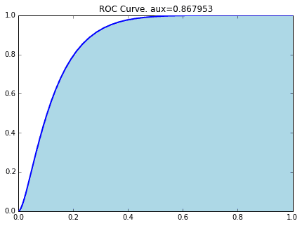
3-2. ROC and AUC

I will explain the index called AUC. This can be derived from the ROC (Receiver Operating Characteristic) curve, but in the previous article,

[Statistics] Understand what an ROC curve is by animation.

Please refer to here for detailed explanations in.

The area under the ROC curve is AUC (Area Under the Curve). (That's right ...: sweat_smile :)

prob = clf.predict_proba(X_test)[:,1]
fpr, tpr, thresholds= roc_curve(y_test, prob)

plt.figure(figsize=(8,6))
plt.plot(fpr, tpr)
plt.title("ROC curve")
plt.xlabel("False Positive Rate")
plt.ylabel("True Positive Rate")
plt.show()

The ROC curve when the Titanic data is classified by SVM (Linear Kernel) is as follows.

#Calculation of AUC
precision, recall, thresholds = precision_recall_curve(y_test, prob)
area = auc(recall, precision)
print "Area Under Curve: {0:.3f}".format(area)

`out`


Area Under Curve: 0.800

reference

WEB 　Scikit Learn User Guide 3. Model selection and evaluation 　　　http://scikit-learn.org/stable/model_selection.html

** Books ** "First pattern recognition" Yuzo Hirai "Introduction to Machine Learning for Language Processing" Manabu Okumura

[PYTHON] [Machine learning] Summary and execution of model evaluation / indicators (w / Titanic dataset)

0. Dataset "Titanic"

First of all, preprocessing and data import

1. Dataset split

1-1. Holdout method

out

out

out

1-2. Cross Validation (CV): Stratified k-fold

out

out

Try to run

out

2. How to find better hyperparameters

out

out

out

3. Evaluation index

Correct answer rate [Accuracy]

Precision rate [Precision]

Recall rate [Recall]

F value (F-measure)

3-1. Try to calculate

out

3-2. ROC and AUC

out

reference

`out`

`out`

`out`

`out`

`out`

`out`

`out`

`out`

`out`

`out`

`out`