[PYTHON] National Medical AI Contest 2020 1st place solution

0. Introduction

I won the medical table data competition called National Medical AI Contest 2020 sponsored by Osaka University AI & Machine learning Society (AIMS) (1st place, top 6%), so I will post the solution.

As you may know from the articles so far, I am not very good at table data competition because I specialize in image data. Please note that there may be some mistakes and irrational parts.

In addition, this article is basically written for those who participated in the competition. There is no explanation about specific column names and features, so you can skip those parts. (The technical part is explained in some detail!)

Similarly, since it was a private competition, you cannot access the competition site other than the participants.

1. About the competition

1-1. Outline of the competition

The competition is a table data competition for predicting death of COVID-19 patients. We will analyze the data on the risk factors (location, presence or absence of pneumonia, age, etc.) that may lead to a given death, and create and submit a model. The competition period is very short, 2 days (9/26 14:00 ~ 9/27 12:00), and the key is how fast inference, implementation, and optimization can be performed. .. In addition, participation in the competition was limited to students.

1-2. Evaluation index

The evaluation index is the area under the ROC curve. This evaluation index has already been explained in the following article, so I will omit it. [Melanoma competition-Area under ROC curve](https://qiita.com/tachyon777/items/05e7d35b7e0b53ef03dd#1-2%E8%A9%95%E4%BE%A1%E6%8C%87%E6%A8% 99)

1-3. Data set

Dataset is simple ・ Train.csv ・ Test.csv ・ Sample_submission.csv It consists of three parts. It will be learned by train, predicted test, and submitted in the form of sample_submission.

Regarding the data contents, there were the following. ・ Patient's address (details) ·age ・ Location of hospital ・ Patient's birthplace ・ Facilities where patients were treated ・ Do you have a history of contact with other COVID patients? ・ PCR test results ·pneumonia ・ Date of onset ・ Hospitalization date (consultation date) ・ Intubation ・ Hospitalization or outpatient ・ Presence or absence of chronic renal failure, diabetes, hypertension, cardiovascular disease, asthma, and other underlying diseases

Since the result of predicting test.csv is actually reflected in LeaderBoard (not Code Competition), the amount given as test data is large, and it was thought that methods such as Pseudo Labeling would be effective.

2.EDA I didn't have to do anything. That's because Akiyama, who runs the competition, released a notebook that combines EDA and baseline at the start of the competition, and almost all the necessary information was available. In particular, the score of LightGBM's feature_importance was listed, and the rest was just to implement the model. With very easy-to-understand data analysis, I was able to start implementing the model immediately.

3. Theory

In theory, I will explain the key method of my solution this time.

3-1. Target Encoding Target encoding is a method that uses the "mean value of the correct label of the category" itself as a feature in a category variable. Since the correct label itself is used indirectly as a feature, it is necessary to be careful about leaks and implementation is quite troublesome. The reason I needed this technique this time was because there was a categorical variable called "place_patient_live2" with 477 categories. Normally, when using a categorical variable in NN, it is processed by OneHotEncoding (in GBDT, the categorical variable can be used as it is), but if you create 477 columns and only one of them makes sense, many You can see that the column becomes a useless feature (= sparse matrix) Therefore, it was necessary to significantly reduce the number of columns (477 → 1) by using target encoding so that learning could be performed efficiently. In fact, the latter was significantly more accurate in my model when trained with OneHotEncoding and with target encoding.

3-2. Pseudo Labeling Pseudo Labeling is a semi-supervised learning method. We aim to improve accuracy by learning not only training data but also test data. First, train the training data with a normal model, evaluate the test data, and output the predicted value, but use this predicted value as it is as the label of the test data, and train again with training + test data from 0. I will. As a result, if the training prediction result is correct to some extent, the diversity of the test data can be obtained. When using this method, it is necessary to give enough test data, and it cannot be used in competitions such as Code Competition where almost no test data is given. You also need to be careful about the amount of test data you use, and it is said that it is better to use an amount such that train: test = 2: 1.

By using this method, the accuracy of a single model can be determined.

• Public LB 0.96696→0.96733 And achieved a significant improvement in accuracy.

This time, we actually used the output results of the NN model and LGBM model ensembles as labels for the test data.

4. Verification

4-1. Policy

Originally, before this competition started, I had a rough idea that it would be table data, so let's go with the flow of EDA → creating a baseline with LightGBM → extracting the weight of features → implementing NN! However, at the start of the competition, the implementation by EDA and LightGBM by Mr. Akiyama, the operation, and the weight of the feature amount were released, so there was not much to do anymore. (I was looking forward to implementing it from scratch, so it's a bit disappointing for those who have experienced competition ...)

Now that we know the accuracy of LightGBM, we implemented the linear model with Pytorch as a baseline. (For the time being, the policy was to start creating features with LightGBM as it is, but since I don't have much knowledge about Feature Engineering, I suddenly started creating NN.)

4-2. Selection and usage of features to be used

As for the features to be used, I used almost all of the LGBM models that have already been released. Since the method of creating the feature amount to be applied is different for each, the one used at the baseline is roughly described below.

** ・ Standardization ** Standardization. Scale to mean 0, variance 1.

standard_cols = [
    "age",
    "entry_-_symptom_date",
    "entry_date_count",
    "date_symptoms",
    "entry_date",
]

** ・ Onehot Encoding ** Handling of categorical variables. Create as many columns as there are categories, and set 1 for that column and 0 for the others.

onehot_cols = [
    "place_hospital",
    "place_patient_birth",
    "type_hospital",
    "contact_other_covid",
    "test_result",
    "pneumonia",
    "intubed",
    "patient_type",
    "chronic_renal_failure",
    "diabetes",
    "icu",
    "obesity",
    "immunosuppression",
    "sex",
    "other_disease",
    "pregnancy",
    "hypertension",
    "cardiovascular",
    "asthma",
    "tobacco",
    "copd",
]

** ・ Target Encoding ** A method that uses the average of correct labels for the entire category as a feature target_E_cols = ["place_patient_live2"]

・ Data related to dates First, change the data given as a date (2020/09/26) to data that can be considered as a continuous value (example: 9/27: 1, 9/28: 2 when 9/26 is 0). .. After that, min_max_encoding is performed with the maximum value set to 1 and the minimum value set to 0.

4-3. Baseline

name : medcon2020_tachyon_baseline
about : simple NN baseline
model : Liner Model
batch : 32
epoch : 20
criterion : BCEWithLogitsLoss
optimizer : Adam
init_lr : 1e-2
scheduler: CosineAnnealingLR
data : plane
preprocess : OnehotEncoding,Standardization,Target Encoding
train_test_split : StratifiedKFold, k=5

Public LB : 0.96575

4-4. LightGBM model

For the features, Akiyama's Feature Engineering results were used as they were, and parameter tuning was performed by applying Optuna. result,

Akiyama's baseline: Public LB0.96636
Model using Optuna: Public LB0.96635

Since almost the same result was obtained, it can be said that this baseline was a fairly complete model. However, since the model has different parameters to some extent, the ensemble effect (improvement of accuracy due to diversity) can be expected to some extent.

4-5. Ensemble submission

After adjusting the baseline parameters of 4-2 and getting some accuracy, I first submitted one NN model and Akiyama's baseline model average ensemble.

※Public LB

NN alone: 0.96696
LGBM alone: 0.96636
Average Ensembling : 0.96738

It is an unexpected improvement in accuracy. Since the algorithms of NN and GBDT are completely different, it is considered that the score has increased significantly. At that time, I was ranked number one in Butchigiri.

4-6.Pseudo Labeling On the second day (final day), we implemented Pseudo Labeling explained in 3. Theory. There may have been a quicker way to improve accuracy, but I could only think of this ...

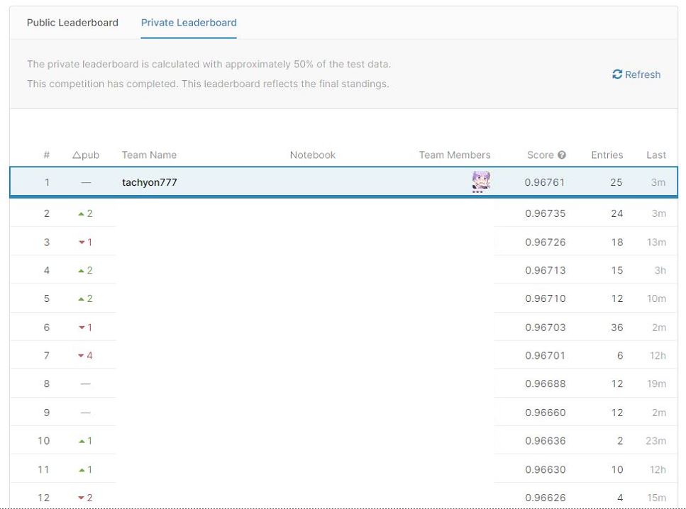
Before implementation of Pseudo Labeling Average Ensemble Score: Private: 0.96753 Public: 0.96761 After implementing Pseudo Labeling Average Ensemble Score: ** Private: 0.96761 ** Public: 0.96768

In the end, I chose these two as the final submission. As a result, the latter became the winning model.

4-7.Pipeline Excuse me for the PowerPoint slides, but I ended up with the following pipeline.

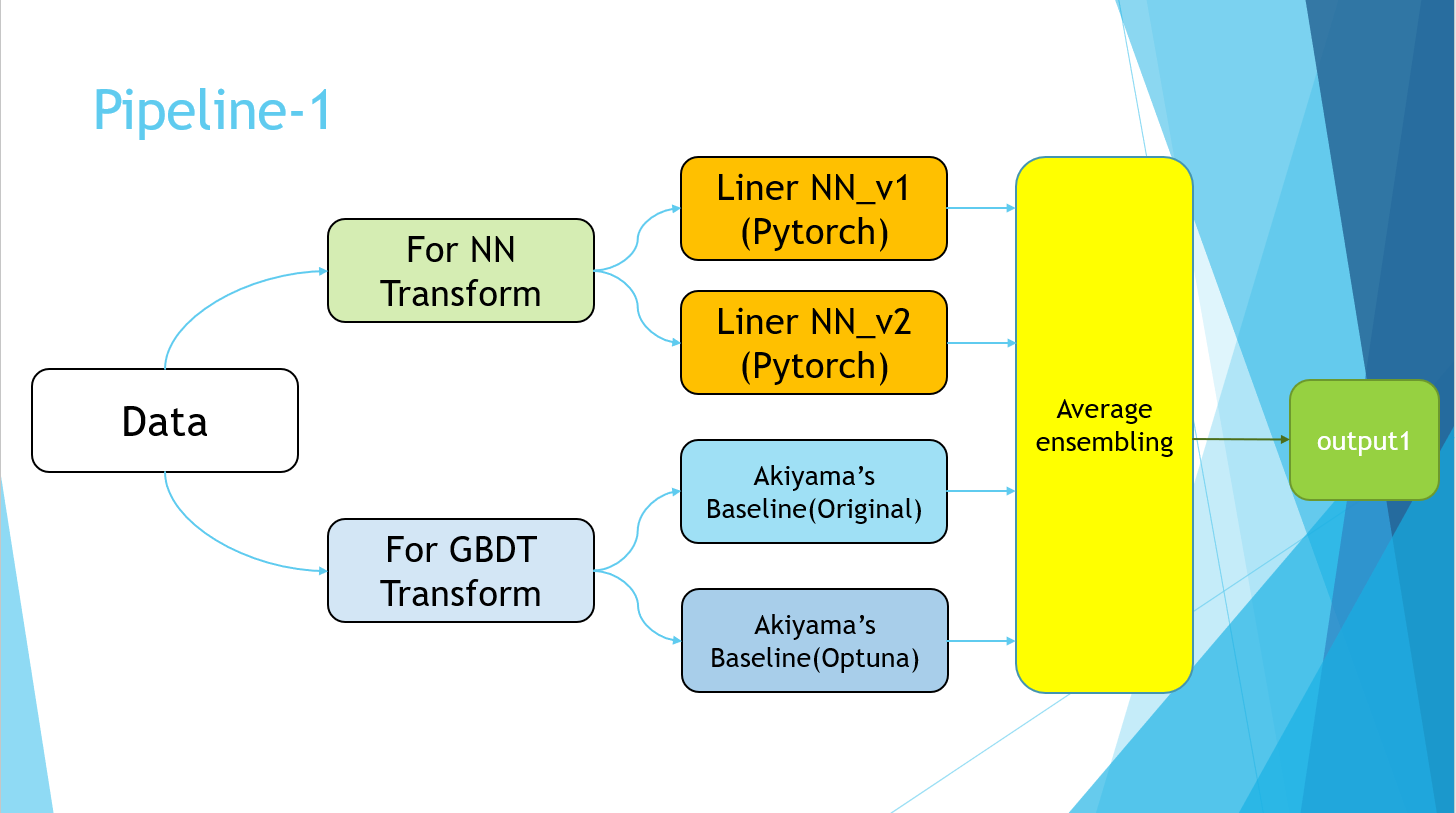
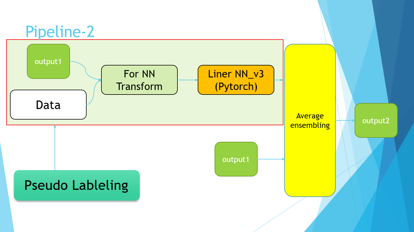
The Pipeline-2 part simply refers to the implementation of Pseudo Labeling. Finally, the average values of the four models of Pipeline-1 and the models trained using the Pseudo Labeling data of Pipeline-2 were taken.

5. Result

Won. (Have you ever won a championship in your life ...?) As for the method, I feel that I have done it perfectly, and I have a sense of accomplishment. On the second day, I was always in first place and worried that I wouldn't be overtaken, so I felt more relieved than happy ...

6. Consideration

Since this is a private contest, I will refrain from raising the solution of other people. Another thing I wanted to try is from the top ・ Creation of features ・ Cat boost ・ Hyperparameter adjustment of NN model It's like that. If kaggle actually held a competition with this data, my score would be below the bronze medal, so I think there is still room for improvement.

7. At the end

Thank you to all the organizers, including the Osaka University AI & Machine learning Society (AIMS), the presenters on the first day, and the contest participants! I hope my solution is helpful as much as possible.

8. References

1. Daisuke Kadowaki Takashi Sakata Keisuke Hosaka Yuji Hiramatsu Winning with Kaggle Data analysis technology Gijutsu-Hyoronsha 2019