[PYTHON] Korrelationskoeffizient MIC, der nichtlineare Beziehungen verarbeiten kann, und Hilbert-Schmidt-Unabhängigkeitstest HSIC
Der Pearson-Korrelationskoeffizient ist ein bekannter Index zur Messung der Unabhängigkeit von Variablen. Es handelt sich jedoch um einen Index, der sich mit linearen (linearen) Beziehungen befasst, und wenn eine U-förmige Beziehung wie eine quadratische Funktion vorliegt, wird er als "keine Korrelation" beurteilt. MIC und HSIC sind als Indikatoren für den Umgang mit solchen nichtlinearen Beziehungen bekannt, daher habe ich versucht, das Python-Paket zu verwenden.
Der gesamte unten stehende Code wurde mit Google Colaboratory getestet.
Python-Paket zur Berechnung des maximalen Informationskoeffizienten (MIC)
Sie können die Installation wie folgt durchführen:
!pip install minepy
Bereiten Sie sich nach der Installation wie folgt vor.
from minepy import MINE
mine = MINE()
Python-Paket zur Berechnung des HSIC (Hilbert-Schmidt Independence Criterion)
Git-Klon wie folgt:
!git clone https://github.com/amber0309/HSIC.git
Bereiten Sie wie folgt vor.
from HSIC.HSIC import hsic_gam
Lineare Funktion
Lassen Sie uns zunächst die lineare Funktion untersuchen.
%matplotlib inline
import matplotlib.pyplot as plt
import numpy as np

X = np.linspace(-1, 1, 51)
Y = X
plt.scatter(X, Y)

Der Pearson-Korrelationskoeffizient ist
np.corrcoef(X, Y)[0, 1]
1.0
MIC ist
mine.compute_score(X, Y)
mine.mic()
0.9999999999999998
Je größer der nächste Wert ist, desto geringer ist die Unabhängigkeit von HSSC, und je kleiner der Wert ist, desto höher ist die Unabhängigkeit.
testStat, thresh = hsic_gam(X.reshape(len(X), 1), Y.reshape(len(Y), 1))
testStat / thresh
22.610487654066624
Fügen wir der linearen Funktion Rauschen hinzu.
import numpy as np

X = np.linspace(-1, 1, 51)
Y = X + np.random.rand(51,)
plt.scatter(X, Y)

Der Pearson-Korrelationskoeffizient ist
np.corrcoef(X, Y)[0, 1]
0.9018483832673769
MIC ist
mine.compute_score(X, Y)
mine.mic()
0.9997226475394071
HSIC
testStat, thresh = hsic_gam(X.reshape(len(X), 1), Y.reshape(len(Y), 1))
testStat / thresh
13.706487127525389
Berechnen wir, wie sich der Pearson-Korrelationskoeffizient ändert, wenn das Rauschen nach und nach zunimmt.
D = []
C = []
for d in range(100):
    X = np.linspace(-1, 1, 51)
    Y = X + np.random.rand(51,) * d / 10
    D.append(d)
    C.append(np.corrcoef(X, Y)[0, 1])

plt.plot(D, C)

In ähnlicher Weise berechnen wir, wie sich die MIC ändert, wenn das Rauschen nach und nach erhöht wird.
D = []
C = []
for d in range(100):
    X = np.linspace(-1, 1, 51)
    Y = X + np.random.rand(51,) * d / 10
    D.append(d)
    mine.compute_score(X, Y)
    C.append(mine.mic())

plt.plot(D, C)
In ähnlicher Weise berechnen wir, wie sich der HSIC ändert, wenn der Geräuschpegel nach und nach erhöht wird.
D = []
C = []
for d in range(100):
    X = np.linspace(-1, 1, 51)
    Y = X + np.random.rand(51,) * d / 10
    D.append(d)
    testStat, thresh = hsic_gam(X.reshape(len(X), 1), Y.reshape(len(Y), 1))
    C.append(testStat / thresh)

plt.plot(D, C)

quadratische Funktion
Als nächstes kommt die quadratische Funktion.
import numpy as np

X = np.linspace(-1, 1, 51)
Y = X**2
plt.scatter(X, Y)

Der Pearson-Korrelationskoeffizient ist
np.corrcoef(X, Y)[0, 1]
-2.3862043230836297e-17
MIC ist
mine.compute_score(X, Y)
mine.mic()
0.9997226475394071
HSIC
testStat, thresh = hsic_gam(X.reshape(len(X), 1), Y.reshape(len(Y), 1))
testStat / thresh
9.285886928766184
Fügen wir Rauschen hinzu.
X = np.linspace(-1, 1, 51)
Y = X**2 + np.random.rand(51,)
plt.scatter(X, Y)

Der Pearson-Korrelationskoeffizient ist
np.corrcoef(X, Y)[0, 1]
0.04693076570744622
MIC ist
mine.compute_score(X, Y)
mine.mic()
0.5071787519579662
HSIC
testStat, thresh = hsic_gam(X.reshape(len(X), 1), Y.reshape(len(Y), 1))
testStat / thresh
5.247036645612692
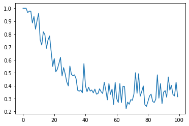
Berechnen wir, wie sich der Pearson-Korrelationskoeffizient ändert, wenn das Rauschen nach und nach zunimmt.
D = []
C = []
for d in range(100):
    X = np.linspace(-1, 1, 51)
    Y = X**2 + np.random.rand(51,) * d / 10
    D.append(d)
    C.append(np.corrcoef(X, Y)[0, 1])

plt.plot(D, C)

In ähnlicher Weise berechnen wir, wie sich die MIC ändert, wenn das Rauschen nach und nach erhöht wird.
D = []
C = []
for d in range(100):
    X = np.linspace(-1, 1, 51)
    Y = X**2 + np.random.rand(51,) * d / 10
    D.append(d)
    mine.compute_score(X, Y)
    C.append(mine.mic())

plt.plot(D, C)

In ähnlicher Weise berechnen wir, wie sich der HSIC ändert, wenn der Geräuschpegel nach und nach erhöht wird.
D = []
C = []
for d in range(100):
    X = np.linspace(-1, 1, 51)
    Y = X**2 + np.random.rand(51,) * d / 10
    D.append(d)
    testStat, thresh = hsic_gam(X.reshape(len(X), 1), Y.reshape(len(Y), 1))
    C.append(testStat / thresh)

plt.plot(D, C)

Es ist ersichtlich, dass der Pearson-Korrelationskoeffizient die Beziehung der quadratischen Funktion nicht erfassen konnte, während sowohl MIC als auch HSIC erfasst werden konnten. Sie können auch sehen, dass das MIC von kleinen Geräuschen weitgehend unberührt bleibt.
Trigonometrische Funktion
Schauen wir uns auch die Dreiecksfunktion an.
import numpy as np

X = np.linspace(-1, 1, 51)
Y = np.sin((X)*np.pi*2)
plt.scatter(X, Y)

Der Pearson-Korrelationskoeffizient ist
np.corrcoef(X, Y)[0, 1]
-0.37651692742033543
MIC ist
mine.compute_score(X, Y)
mine.mic()
0.9997226475394071
HSIC
testStat, thresh = hsic_gam(X.reshape(len(X), 1), Y.reshape(len(Y), 1))
testStat / thresh
3.212604441715373
Fügen wir Rauschen hinzu.
import numpy as np

X = np.linspace(-1, 1, 51)
Y = np.sin((X+0.25)*np.pi*2) + np.random.rand(51,)
plt.scatter(X, Y)

Der Pearson-Korrelationskoeffizient ist
np.corrcoef(X, Y)[0, 1]
0.049378342546505014
MIC ist
mine.compute_score(X, Y)
mine.mic()
0.9997226475394071
HSIC
testStat, thresh = hsic_gam(X.reshape(len(X), 1), Y.reshape(len(Y), 1))
testStat / thresh
1.3135420547013614
Untersuchen Sie den Effekt der Erhöhung des Rauschens. Der Pearson-Korrelationskoeffizient ist
D = []
C = []
for d in range(100):
    X = np.linspace(-1, 1, 51)
    Y = np.sin((X+0.25)*np.pi*2) + np.random.rand(51,) * d / 10
    D.append(d)
    C.append(np.corrcoef(X, Y)[0, 1])

plt.plot(D, C)

MIC ist
D = []
C = []
for d in range(100):
    X = np.linspace(-1, 1, 51)
    Y = np.sin((X+0.25)*np.pi*2) + np.random.rand(51,) * d / 10
    D.append(d)
    mine.compute_score(X, Y)
    C.append(mine.mic())

plt.plot(D, C)

HSIC
D = []
C = []
for d in range(100):
    X = np.linspace(-1, 1, 51)
    Y = np.sin((X+0.25)*np.pi*2) + np.random.rand(51,) * d / 10
    D.append(d)
    testStat, thresh = hsic_gam(X.reshape(len(X), 1), Y.reshape(len(Y), 1))
    C.append(testStat / thresh)

plt.plot(D, C)

Es wurde erwartet, dass der Pearson-Korrelationskoeffizient die Beziehung der Dreiecksfunktion zum Rauschen nicht erfassen konnte, aber es scheint, dass HSIC ebenfalls abgefallen ist. Unter ihnen war ich überrascht, dass MIC die Beziehung erkennen konnte.
Sigmaid-Funktion
Schließlich gibt es die Sigmoidfunktion.
import numpy as np

X = np.linspace(-1, 1, 51)
Y = 1 / (1 + np.exp(-X*10))
plt.scatter(X, Y)

Der Pearson-Korrelationskoeffizient ist
np.corrcoef(X, Y)[0, 1]
0.9354020629807919
MIC ist
mine.compute_score(X, Y)
mine.mic()
0.9999999999999998
HSIC
testStat, thresh = hsic_gam(X.reshape(len(X), 1), Y.reshape(len(Y), 1))
testStat / thresh
27.433932271008874
Fügen wir Rauschen hinzu.
import numpy as np

X = np.linspace(-1, 1, 51)
Y = 1 / (1 + np.exp(-X*10)) + np.random.rand(51,)
plt.scatter(X, Y)

Der Pearson-Korrelationskoeffizient ist
np.corrcoef(X, Y)[0, 1]
0.7994507640548881
MIC ist
mine.compute_score(X, Y)
mine.mic()
0.9997226475394071
HSIC
testStat, thresh = hsic_gam(X.reshape(len(X), 1), Y.reshape(len(Y), 1))
testStat / thresh
12.218008194240534
Lassen Sie uns sehen, wie sich das Rauschen erhöht. Der Pearson-Korrelationskoeffizient ist
D = []
C = []
for d in range(100):
    X = np.linspace(-1, 1, 51)
    Y = 1 / (1 + np.exp(-X*10)) + np.random.rand(51,) * d / 10
    D.append(d)
    C.append(np.corrcoef(X, Y)[0, 1])

plt.plot(D, C)

MIC ist
D = []
C = []
for d in range(100):
    X = np.linspace(-1, 1, 51)
    Y = 1 / (1 + np.exp(-X*10)) + np.random.rand(51,) * d / 10
    D.append(d)
    mine.compute_score(X, Y)
    C.append(mine.mic())

plt.plot(D, C)

HSIC
D = []
C = []
for d in range(100):
    X = np.linspace(-1, 1, 51)
    Y = 1 / (1 + np.exp(-X*10)) + np.random.rand(51,) * d / 10
    D.append(d)
    testStat, thresh = hsic_gam(X.reshape(len(X), 1), Y.reshape(len(Y), 1))
    C.append(testStat / thresh)

plt.plot(D, C)

Alle Indikatoren können die Beziehung erkennen, aber in Bezug auf die Rauschbeständigkeit scheint MIC am stärksten zu sein.
Es ist ein individueller Eindruck
MIC MIC!