Pearson's correlation coefficient is a well-known index for measuring the independence of variables. However, it is an index that deals with linear (linear) relationships, and when there is a U-shaped relationship such as a quadratic function, it is judged as "no correlation". MIC and HSIC are known as indicators for dealing with such non-linear relationships, so I tried using the Python package.

All of the code below has been tested on Google Colaboratory.

A Python package that calculates the Maximal Information Coefficient (MIC)

You can pip install as follows:

!pip install minepy

After installation, prepare as follows.

from minepy import MINE
mine = MINE()

A Python package that calculates HSIC (Hilbert-Schmidt Independence Criterion)

Git clone as follows:

!git clone https://github.com/amber0309/HSIC.git

Prepare as follows.

from HSIC.HSIC import hsic_gam

Linear function

First, let's examine the linear function.

%matplotlib inline
import matplotlib.pyplot as plt
import numpy as np

X = np.linspace(-1, 1, 51)
Y = X
plt.scatter(X, Y)

Pearson's correlation coefficient is

np.corrcoef(X, Y)[0, 1]

1.0

MIC is

mine.compute_score(X, Y)
mine.mic()

0.9999999999999998

HSSC is said to have lower independence as the next value is larger, and higher independence as the next value is smaller.

testStat, thresh = hsic_gam(X.reshape(len(X), 1), Y.reshape(len(Y), 1))
testStat / thresh

22.610487654066624

Let's add noise to the linear function.

import numpy as np

X = np.linspace(-1, 1, 51)
Y = X + np.random.rand(51,)
plt.scatter(X, Y)

Pearson's correlation coefficient is

np.corrcoef(X, Y)[0, 1]

0.9018483832673769

MIC is

mine.compute_score(X, Y)
mine.mic()

0.9997226475394071

HSIC

testStat, thresh = hsic_gam(X.reshape(len(X), 1), Y.reshape(len(Y), 1))
testStat / thresh

13.706487127525389

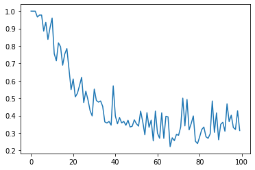
Let's calculate how Pearson's correlation coefficient changes as the amount of noise is increased little by little.

D = []
C = []
for d in range(100):
    X = np.linspace(-1, 1, 51)
    Y = X + np.random.rand(51,) * d / 10
    D.append(d)
    C.append(np.corrcoef(X, Y)[0, 1])

plt.plot(D, C)

Similarly, let's calculate how the MIC changes as the noise level is increased little by little.


D = []
C = []
for d in range(100):
    X = np.linspace(-1, 1, 51)
    Y = X + np.random.rand(51,) * d / 10
    D.append(d)
    mine.compute_score(X, Y)
    C.append(mine.mic())

plt.plot(D, C)

Similarly, let's calculate how the HSIC changes as the noise level is increased little by little.

D = []
C = []
for d in range(100):
    X = np.linspace(-1, 1, 51)
    Y = X + np.random.rand(51,) * d / 10
    D.append(d)
    testStat, thresh = hsic_gam(X.reshape(len(X), 1), Y.reshape(len(Y), 1))
    C.append(testStat / thresh)

plt.plot(D, C)

quadratic function

Next is the quadratic function.

import numpy as np

X = np.linspace(-1, 1, 51)
Y = X**2
plt.scatter(X, Y)

Pearson's correlation coefficient is

np.corrcoef(X, Y)[0, 1]

-2.3862043230836297e-17

MIC is

mine.compute_score(X, Y)
mine.mic()

0.9997226475394071

HSIC

testStat, thresh = hsic_gam(X.reshape(len(X), 1), Y.reshape(len(Y), 1))
testStat / thresh

9.285886928766184

Let's add noise.

X = np.linspace(-1, 1, 51)
Y = X**2 + np.random.rand(51,)
plt.scatter(X, Y)

Pearson's correlation coefficient is

np.corrcoef(X, Y)[0, 1]

0.04693076570744622

MIC is

mine.compute_score(X, Y)
mine.mic()

0.5071787519579662

HSIC

testStat, thresh = hsic_gam(X.reshape(len(X), 1), Y.reshape(len(Y), 1))
testStat / thresh

5.247036645612692

Let's calculate how Pearson's correlation coefficient changes as the amount of noise is increased little by little.


D = []
C = []
for d in range(100):
    X = np.linspace(-1, 1, 51)
    Y = X**2 + np.random.rand(51,) * d / 10
    D.append(d)
    C.append(np.corrcoef(X, Y)[0, 1])

plt.plot(D, C)

Similarly, let's calculate how the MIC changes as the noise level is increased little by little.


D = []
C = []
for d in range(100):
    X = np.linspace(-1, 1, 51)
    Y = X**2 + np.random.rand(51,) * d / 10
    D.append(d)
    mine.compute_score(X, Y)
    C.append(mine.mic())

plt.plot(D, C)

Similarly, let's calculate how the HSIC changes as the noise level is increased little by little.

D = []
C = []
for d in range(100):
    X = np.linspace(-1, 1, 51)
    Y = X**2 + np.random.rand(51,) * d / 10
    D.append(d)
    testStat, thresh = hsic_gam(X.reshape(len(X), 1), Y.reshape(len(Y), 1))
    C.append(testStat / thresh)

plt.plot(D, C)

It can be seen that Pearson's correlation coefficient cannot detect the relationship of the quadratic function, while both MIC and HSIC can be detected. You can also see that the MIC will be largely unaffected by small noise.

Trigonometric function

Let's also look at trigonometric functions.

import numpy as np

X = np.linspace(-1, 1, 51)
Y = np.sin((X)*np.pi*2)
plt.scatter(X, Y)

Pearson's correlation coefficient is

np.corrcoef(X, Y)[0, 1]

-0.37651692742033543

MIC is

mine.compute_score(X, Y)
mine.mic()

0.9997226475394071

HSIC

testStat, thresh = hsic_gam(X.reshape(len(X), 1), Y.reshape(len(Y), 1))
testStat / thresh

3.212604441715373

Let's add noise.

import numpy as np

X = np.linspace(-1, 1, 51)
Y = np.sin((X+0.25)*np.pi*2) + np.random.rand(51,)
plt.scatter(X, Y)

Pearson's correlation coefficient is

np.corrcoef(X, Y)[0, 1]

0.049378342546505014

MIC is

mine.compute_score(X, Y)
mine.mic()

0.9997226475394071

HSIC

testStat, thresh = hsic_gam(X.reshape(len(X), 1), Y.reshape(len(Y), 1))
testStat / thresh

1.3135420547013614

Investigate the effect of increasing the noise. Pearson's correlation coefficient is

D = []
C = []
for d in range(100):
    X = np.linspace(-1, 1, 51)
    Y = np.sin((X+0.25)*np.pi*2) + np.random.rand(51,) * d / 10
    D.append(d)
    C.append(np.corrcoef(X, Y)[0, 1])

plt.plot(D, C)

MIC is

D = []
C = []
for d in range(100):
    X = np.linspace(-1, 1, 51)
    Y = np.sin((X+0.25)*np.pi*2) + np.random.rand(51,) * d / 10
    D.append(d)
    mine.compute_score(X, Y)
    C.append(mine.mic())

plt.plot(D, C)

HSIC

D = []
C = []
for d in range(100):
    X = np.linspace(-1, 1, 51)
    Y = np.sin((X+0.25)*np.pi*2) + np.random.rand(51,) * d / 10
    D.append(d)
    testStat, thresh = hsic_gam(X.reshape(len(X), 1), Y.reshape(len(Y), 1))
    C.append(testStat / thresh)

plt.plot(D, C)

It was expected that Pearson's correlation coefficient could not detect the relationship of trigonometric functions with noise, but it seems that HSIC has also dropped out. Among them, I was surprised that MIC was able to detect the relationship.

Sigmoid function

Finally, there is the sigmoid function.

import numpy as np

X = np.linspace(-1, 1, 51)
Y = 1 / (1 + np.exp(-X*10))
plt.scatter(X, Y)

Pearson's correlation coefficient is

np.corrcoef(X, Y)[0, 1]

0.9354020629807919

MIC is

mine.compute_score(X, Y)
mine.mic()

0.9999999999999998

HSIC

testStat, thresh = hsic_gam(X.reshape(len(X), 1), Y.reshape(len(Y), 1))
testStat / thresh

27.433932271008874

Let's add noise.

import numpy as np

X = np.linspace(-1, 1, 51)
Y = 1 / (1 + np.exp(-X*10)) + np.random.rand(51,)
plt.scatter(X, Y)

Pearson's correlation coefficient is

np.corrcoef(X, Y)[0, 1]

0.7994507640548881

MIC is

mine.compute_score(X, Y)
mine.mic()

0.9997226475394071

HSIC

testStat, thresh = hsic_gam(X.reshape(len(X), 1), Y.reshape(len(Y), 1))
testStat / thresh

12.218008194240534

Let's see the effect of increasing the noise. Pearson's correlation coefficient is


D = []
C = []
for d in range(100):
    X = np.linspace(-1, 1, 51)
    Y = 1 / (1 + np.exp(-X*10)) + np.random.rand(51,) * d / 10
    D.append(d)
    C.append(np.corrcoef(X, Y)[0, 1])

plt.plot(D, C)

MIC is

D = []
C = []
for d in range(100):
    X = np.linspace(-1, 1, 51)
    Y = 1 / (1 + np.exp(-X*10)) + np.random.rand(51,) * d / 10
    D.append(d)
    mine.compute_score(X, Y)
    C.append(mine.mic())

plt.plot(D, C)

HSIC


D = []
C = []
for d in range(100):
    X = np.linspace(-1, 1, 51)
    Y = 1 / (1 + np.exp(-X*10)) + np.random.rand(51,) * d / 10
    D.append(d)
    testStat, thresh = hsic_gam(X.reshape(len(X), 1), Y.reshape(len(Y), 1))
    C.append(testStat / thresh)

plt.plot(D, C)

All of the indicators can detect the relationship, but in terms of noise resistance, MIC seems to be the strongest.

It is an individual impression

MIC MIC!

[PYTHON] Correlation coefficient MIC and Hilbert-Schmidt independence test HSIC that can handle non-linear relationships

A Python package that calculates the Maximal Information Coefficient (MIC)

A Python package that calculates HSIC (Hilbert-Schmidt Independence Criterion)

Linear function

quadratic function

Trigonometric function

Sigmoid function

It is an individual impression